A biologist’s checklist for calcium imaging and optogenetic analysis

Andrey Andreev (aandreev@caltech.edu), Daniel Lee (leed@caltech.edu), Erin Berlew (erin.berlew@gmail.com)

Engaging in optogenetic experiments – understanding understated complexities

Optogenetics, calcium imaging, and modern microscopy provide a powerful approach to uncover new biological phenomena and explore cellular and molecular mechanisms in ways that are both visual and quantitative. Paired properly, optogenetic approaches combined with calcium imaging can determine functional relationships within biological circuits. For example, stimulating or inhibiting neural populations, and subsequently recording neural activity, allows one to examine the presence of epistatic neural relationships. Technological advancement constantly makes these methods more accessible, however, there are a number of understated complexities involved with these types of imaging-based experiments. Successful application of optogenetics requires good experimental design, controls, and proper understanding of microscopy limitations in order to generate clear and easily interpretable data. This is true both at the level of designing one’s own experiments as well as for critically evaluating studies carried out by others.

In a recent class we taught at Caltech, we introduced students to these concept, practical details, and limitations of optogenetic and calcium imaging experiments.  Here we share a brief “checklist” from that class to make it easier for scientists to start their first hands-on optogenetic and calcium imaging experiments (you can download the checklist PDF here: DOI 10.22002/D1.1947).

The text below provides explanation of several of the questions contained in the checklist. Our goal for our readers is to provide a set of questions that needs to be considered, and ideally answered, prior to or while engaging in your experiment. Often times, there is not a “best” answer, but we hope to encourage scientists to evaluate options and pick one thoughtfully.

Experiment planning

• Do you have sufficient experimental controls? What positive/negative controls will you use?

Place extra emphasis on the experimental design stage of the planning process. Mapping out the necessary controls is one of the first key steps in generating clear, interpretable data. Optogenetic and calcium imaging experiments in live animals need to control for various experimental artifacts. For example, you should control for potential confounds such as phototoxicity through heat-production [1] and activity artifacts  due to endogenous light-sensitive ion channels that have been reported in the brain and body [2]. Photo-damage can be assessed post-imaging by staining with anti-GFAP or anti-HSP70 antibodies.  While a GFP vector (expressing GFP instead of optogenetic channel) can be useful as a negative control in conjunction with an optogenetic transgene in the experimental condition, it may not cover all relevant experimental artifacts in your experimental design. Additionally, it is helpful to establish criteria for excluding images or cells from your final analysis prior to collecting the data to prevent cherry picking or other skewed data analysis methods.

• Is there spectral overlap between your excitation wavelength and the fluorophores you plan to image?

It is important to ensure that you are not inadvertently exciting your optogenetic probe while capturing baseline dark-state images in your experiment. For example, imaging GFP will stimulate any blue light-sensitive system and result in apparent high dark-state activity, an artifact of the overlap between cyan and blue light emission profiles. It is best to verify that there is no overlap on the microscope via a power meter rather than relying on theoretical calculations as filter cubes, laser lines, and excitation pulse widths differ from setup to setup.

• Do you plan to deal with motion artifacts or occlusion by blood vessels when performing live imaging of animals? Do you plan to normalize GCaMP expression by using additional fluorescent markers? 

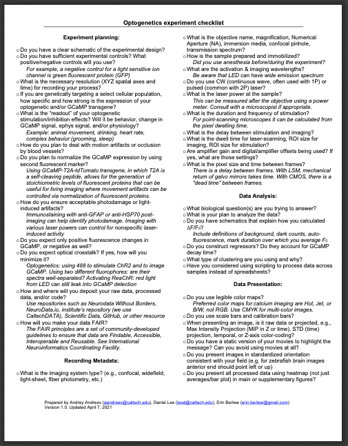
Live imaging in animals is used to identify the cellular basis of behavioral or physiological processes. Motion artifacts or occlusion by blood vessels (discussed in this Twitter thread), however, are an inherent problem that arises from imaging live animals. While there is a number of imaging software functions (such as Fiji plugins) that can help spatially track moving or occluded regions of interests, methodological approaches can aid in ascertaining whether changes in GCaMP signals are due to real changes in calcium signaling, and ostensibly neural activity, or conversely because of movement artifacts. While not standard practice yet, we support stoichiometric expression of GCaMP with another fluorescent protein in cellular populations of interest. For example, in our calcium imaging recordings in live animals, we use the GCaMP-T2A-tdTomato transgene [3][4][5] known sometimes as Salsa [6], where GCaMP allows for monitoring calcium levels, while the compound transgene also contains a self-cleaving peptide T2A (or P2A) and tdTomato cassettes which can help to deal with motion artifacts through normalization of GCaMP expression. T2A, a self-cleaving peptide [7], in combination with tdTomato allows for the generation of stoichiometric levels of tdTomato fluorescent proteins that can be useful for in vivo imaging where movement artifacts can be controlled via normalization of GCaMP fluorescent proteins. For example, in previous studies, we utilized GCaMP6s to monitor calcium levels in hypothalamic npvf-expressing neurons and normalized GCaMP6s fluorescence intensity values to tdTomato fluorescence to correct for any changes in transgene expression or movement artifacts during live imaging. Using this stoichiometric co-expression approach of GCaMP with another fluorescent protein allows one to generate more clearly interpretable results.

• Will you deposit your raw and processed data, code?

Regardless of data volume, whether it is just a few MBs or 100s of GB of data you plan to collect, it is important to realize that temporary data storage and subsequent archiving before the publication are essential steps of the experiments. Sensible ways of storing raw data will make processing and analysis easier for you, and your collaborators who will want to have access to it. Perhaps, you will decide to outsource analysis to a colleague. Perhaps you will expand your dataset from few samples to several dozens.

Unfortunately, today universities often don’t offer good solution for data storage. We have to rely on “Dropbox” or USB-drives that prevent sharing data, or build our own storage servers [8]. It might be acceptable to use Dropbox storage for smaller amounts of data. Make sure to separate and keep secured the raw data from any processed data.

Learn about data storage option at your university, as some libraries run data archiving services (such as CaltechDATA). Public repositories such as Neurodata Without Borders [9] and neurodata.io are providing storage solutions for data pre-publication.

Recording metadata

• Do you measure laser power at the sample?

Measuring laser power is essential. Intense laser light, especially in two-photon experiments, is a potential source of photodamage and artifacts. Not only can laser intensity initiate cell damage and restrict experimental duration, but light damage can also induce off-target activity artifacts. Measuring laser power is also important to perform because laser intensity can change due to microscope misalignment (as discussed in this twitter thread). Finally, measuring laser power is important because lasers can degrade with use (as discussed in Focal Plane light-sheet article); a laser power of “20%” may not be the same in absolute value two months from now. Recording and reporting laser power is important for reproducibility and allowing other replicate your experimental protocol.

Recording laser power is not always easy. One way to do it is to place a high-quality power meter with phosphorescent target to see invisible (two-photon) light under that imaging objective, at a distance slightly away from focal plane. We use the Thorlabs power meter, which even available with a “slide” sensor. If that is not possible, the nominal laser power can be recorded (for example, as displayed in microscope’s interface) and objective transmission taken into account. Some objectives have less than 60% transmission at 920nm, for example. Optical elements (lenses, mirrors) also can cause light to lose 1% of power at each surface. Consult your imaging specialist for assistance. When reporting laser power, specify the location of the measurement.

Analysis of the neural activity data

• Do you use scripting to process data across samples instead of spreadsheets?

Spreadsheet software products, such as Excel, are very commonly used in practice for data management. A better alternative is to store the data in appropriate files (for example, using CSV format) and use scripting programming languages such as Python, MATLAB, Ruby, or even R to process and extract results. The main benefit of this approach is reproducibility, and that the original data is not directly modified in the process (what happens when working with spreadsheets). It is much easier to share the results, check the logic (important in cases of normalization), and outsource analysis to colleagues. It is not just the question of sharing post-publication data: analysis through declarative programming will speed up processing of the data and ensure uniformity across multiple experimental samples and conditions.

In addition, consider if it is possible to blind yourself to the experimental condition(s) of each image during the data processing and analysis phase. Renaming images to arbitrary numbers (and keeping track of corresponding numbers in a key!) reduces experimenter bias introduced during image processing and prevents expectation from clouding interpretation of the results.

• Do you have graphics that explain the calculation of ∆F/F0 and/or definitions?

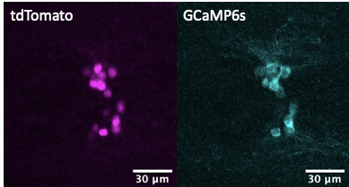
In calcium imaging, the standard way to analyze data is to calculate a ∆F/F0 metric, or relative change in fluorescence in response to some factor. Especially during presentations with live audience, but also in publications, it is crucial to provide a clear explanation of how this calculation was performed. First of all, fluorescence signal recorded by the microscope consists of “dark counts” or other offsets intrinsic to the detector. Secondly, the autofluorescence intensity of the biological sample is added to the photons emitted by the fluorophore (say, GCaMP). These values can vary between experiments and samples. In simple cases, where neural activity is triggered by stimuli, the baseline sensor intensity (F0), is the averaged intensity before the stimulation. Explaining this might be very confusing, so we advise on using a schematic, such as:

The calculation of ∆F/F0 that we propose is:

F = cell_Signal – sample_Background
F₀ = average F for 3-10 frames before the event of interest
∆F/F₀ = (F – F₀)/F₀

DigitalOffset + darkCounts + slide/media autofluorescence = intensity outside the sample

sample_Background = intensity from the sample near cells expressing GCaMP

Data presentation

• Do you use legible colormap?

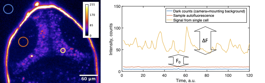
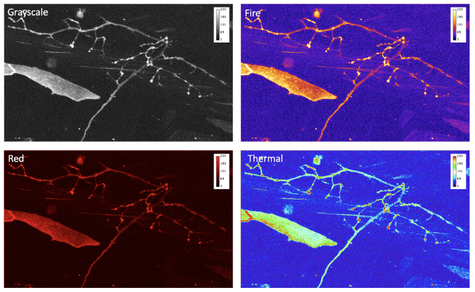
Data that is collected by the microscope is just a set of numbers. To make it more understandable, we can present it through the application of colormaps (also known as lookup tables, or LUT) that transform intensity numbers to screen pixel brightness and color, that in turn is perceived by our eyes [10]. This process of transferring information into numbers can be highly non-linear and depends on multiple factors. Some of these factors are within our control, others such as the difference in color-vision of the audience, needs to be accounted for. Even by dimming the lights in conference room when presenting images, can we help our audience appreciate our invaluable data by choosing proper colormap.

When advising on optimal data presentation, we provide guidance on avoiding the “but it looks good on my screen!” situation. To avoid this scenario, never use Red or Blue or Green primary colors (RGB). Colormaps that allow one to extract more information and that present data more optimally include Cyan-Magenta-Yellow-Key (CMYK, where “key” means black). “Fire” or “Hot” colormaps are often used for single-channel images and movies. Remember, that the best approach can be a conservative one: use grayscale colormap and split multi-channel images into several panels, instead of trying to overlay. To show co-localization of two objects, Cyan and Magenta are good complimentary colors. Your data is more valuable than the few minutes you would spend picking the correct, not “default”, colormap, or splitting data into several panels or figures.

Conclusions

The discussion presented here and the PDF of the checklist (DOI 10.22002/D1.1947) are designed to be a “cheat sheet” or a checklist that can help to make sure that we don’t forget crucial elements of experiments. We plan to use this list ourselves. This list is open for modification for your particular approach, model organism, and/or lab culture. We encourage you to use it while planning experiments, as well as when discussing potential experiments with microscopy specialists. Remember: the current technology of imaging and optogenetics, unfortunately, outpaces the education and training. This growing arsenal of imaging and genetic tools is just too complex to expect everyone performing biomedical research to also be proficient with microscopy and fluorescence. Lastly, consult with your friendly microscopy Core Facility technicians and specialists (and don’t forget to acknowledge the Core Facility’s contribution when you publish).

Authors

Andrey Andreev, PhD — Postdoctoral scholar (Caltech, Prober lab)

Daniel A. Lee, PhD — Senior Research Associate (Caltech, Prober lab)

Erin Berlew — PhD candidate (U Penn, Chow lab)

References

1. Podgorski K, Ranganathan G (2016) Brain heating induced by near-infrared lasers during multiphoton microscopy. J Neurophysiol 116:1012–1023. https://doi.org/10.1152/jn.00275.2016

2. Schmidt E, Oheim M (2020) Infrared Excitation Induces Heating and Calcium Microdomain Hyperactivity in Cortical Astrocytes. Biophys J 119:2153–2165 . https://doi.org/10.1016/j.bpj.2020.10.027

3. Lee DA, Andreev A, Truong TV, Chen A, Hill AJ, Oikonomou G, Pham U, Hong YK, Tran S, Glass L, Sapin V, Engle J, Fraser SE, Prober DA (2017) Genetic and neuronal regulation of sleep by neuropeptide VF. eLife 6:e25727. https://doi.org/10.7554/eLife.25727

4. Lee DA, Liu J, Hong Y, Lane JM, Hill AJ, Hou SL, Wang H, Oikonomou G, Pham U, Engle J, Saxena R, Prober DA (2019) Evolutionarily conserved regulation of sleep by epidermal growth factor receptor signaling. Sci Adv 5:eaax4249 . https://doi.org/10.1126/sciadv.aax4249

5. Lee DA, Oikonomou G, Cammidge T, Andreev A, Hong Y, Hurley H, Prober DA (2020) Neuropeptide VF neurons promote sleep via the serotonergic raphe. eLife 9:e54491 . https://doi.org/10.7554/eLife.54491

6. T-cell calcium dynamics visualized in a ratiometric tdTomato-GCaMP6f transgenic reporter mouse | eLife. https://elifesciences.org/articles/32417

7. Liu Z, Chen O, Wall JBJ, Zheng M, Zhou Y, Wang L, Ruth Vaseghi H, Qian L, Liu J (2017) Systematic comparison of 2A peptides for cloning multi-genes in a polycistronic vector. Sci Rep 7:2193 . https://doi.org/10.1038/s41598-017-02460-2

8. Andreev A, Koo DES (2020) Practical Guide to Storage of Large Amounts of Microscopy Data. Microsc Today 28:42–45 . https://doi.org/10.1017/S1551929520001091

9. Teeters JL, Godfrey K, Young R, Dang C, Friedsam C, Wark B, Asari H, Peron S, Li N, Peyrache A, Denisov G, Siegle JH, Olsen SR, Martin C, Chun M, Tripathy S, Blanche TJ, Harris K, Buzsáki G, Koch C, Meister M, Svoboda K, Sommer FT (2015) Neurodata Without Borders: Creating a Common Data Format for Neurophysiology. Neuron 88:629–634 . https://doi.org/10.1016/j.neuron.2015.10.025

10. Nuñez JR, Anderton CR, Renslow RS (2018) Optimizing colormaps with consideration for color vision deficiency to enable accurate interpretation of scientific data. PLOS ONE 13:e0199239 . https://doi.org/10.1371/journal.pone.0199239

(No Ratings Yet)