Behind the Screen – behind the scenes of setting up a dynamic screening platform
Posted by Sravasti Mukherjee, on 22 November 2021
The Cell Biophysics lab has focused on FRET (Forster Resonance Energy Transfer) as it is a powerful technique to investigate dynamic protein-protein interactions, along with studying almost every aspect of cellular signaling with biosensors. FRET is detected either by ratioing the intensities of the FRET donor and acceptor, or by FLIM (Fluorescence Lifetime Imaging ; recording the donor fluorescence lifetime, i.e., the average time the donor stays in the excited state before returning to the ground state). FLIM is inherently more quantitative than ratiometry because an interaction between donor and acceptor shortens the excited-state lifetime of the donor linearly with FRET efficiency. FLIM recordings are also not affected by differences in sensor expression levels, sensor bleaching, excitation fluctuation and slight misfocusing. Additionally, being a one-channel technique gives it the advantage to avoid artifacts caused by chromatic aberration and sensitivity difference issues between channels, unlike ratio imaging. However, FLIM requires complex and dedicated hardware and has been too slow to record fast dynamic events.
Recently, collaborative efforts of both research labs and leading microscopy manufacturers has led to improved acquisition speed, multi-well handling and extraction of quantitative parameters from FLIM data1-3. Some of our labs’ own developments include implementation of photon efficient and fast FLIM instrumentation, both for confocal4,5 and wide field microscopy6. These improvements enable following large number of cells in real time, with high data content and minimal photo damage (bleaching & phototoxic stress on cells), thus making FLIM a great choice for FRET-based signaling studies.
Our lab also has a long-standing interest in discovering new players in signal transduction pathways, especially in the cAMP (cyclic adenosine monophosphate) pathway. And that definitely pointed towards a genetic screen! However, conventional screening formats are not well suited to read out dynamic phenotypes and thus, most screens focused on static endpoint readouts such as cell viability. Therefore, spatial and temporal information at the single cell level is lost. Using the new FLIM hardware, along with our cAMP biosensor which was tailored specifically for high-efficiency FLIM analysis7,8 we aimed to perform a proof of principle time-lapse genetic screen for dynamic phenotypes. We decided to decipher the contribution of 22 PDE (Phosphodiesterase) isoforms (enzymes that hydrolyze cAMP) in breaking down cAMP.
Designing the assays of the screen:
We first set out to achieve reliable and reproducible cAMP transient in our assays. Using HeLa cells as our study model, we started by elevating cAMP levels with a β2 adrenergic receptor (β-AR) agonist (Isoproterenol) and follow the PDE-mediated cAMP breakdown kinetics. However, after a few pilot experiments we realized that in order to isolate the effects of breakdown by PDEs, we had to rapidly terminate the activity of the β -AR. Hence, we decided to use a β-antagonist (Propranolol) to displace the agonist shortly after stimulation and thereby achieve transient activation of GPCRs. The latter also reduced our total assay time, allowing us to finish the screen within 6-8 hours.
We also tested an alternative approach to achieve transient cAMP elevations, i.e. by UV-release of caged cAMP inside the cell. The biggest challenge we faced here was the leaky nature of caged compounds. Elevation of the baseline cAMP levels in cells treated with caged cAMP was evident and increasingly pronounced when loaded with higher concentrations, but not with longer loading time. Several rounds of tests were needed to optimize loading concentrations such that the baseline elevation was minimal, so as to maintain a high dynamic range of the sensor. To ensure good S/N levels, photo-released cAMP levels had to approach saturating levels of the biosensor. Additional optimizations were required to determine the length of the uncaging pulse – for which we programmed an Arduino-operated automatable shutter-trigger to precisely uncage on the selected frame and to only flash UV in between imaging frames. Interestingly, one can uncage the DMNB cAMP multiple times in the same field of view after clearance by the cell. The caged compound simply diffuses in and regenerates the pool. This could prove handy if one wishes to collect more statistics and fit multiple decay cycles from the same cells. However, these observations did not make it to the final draft of the paper, partly because in such experiments PDE activity could be overestimated in the follow-up pulses of cAMP as the PDEs are already working at full capacity.
Imaging conditions:
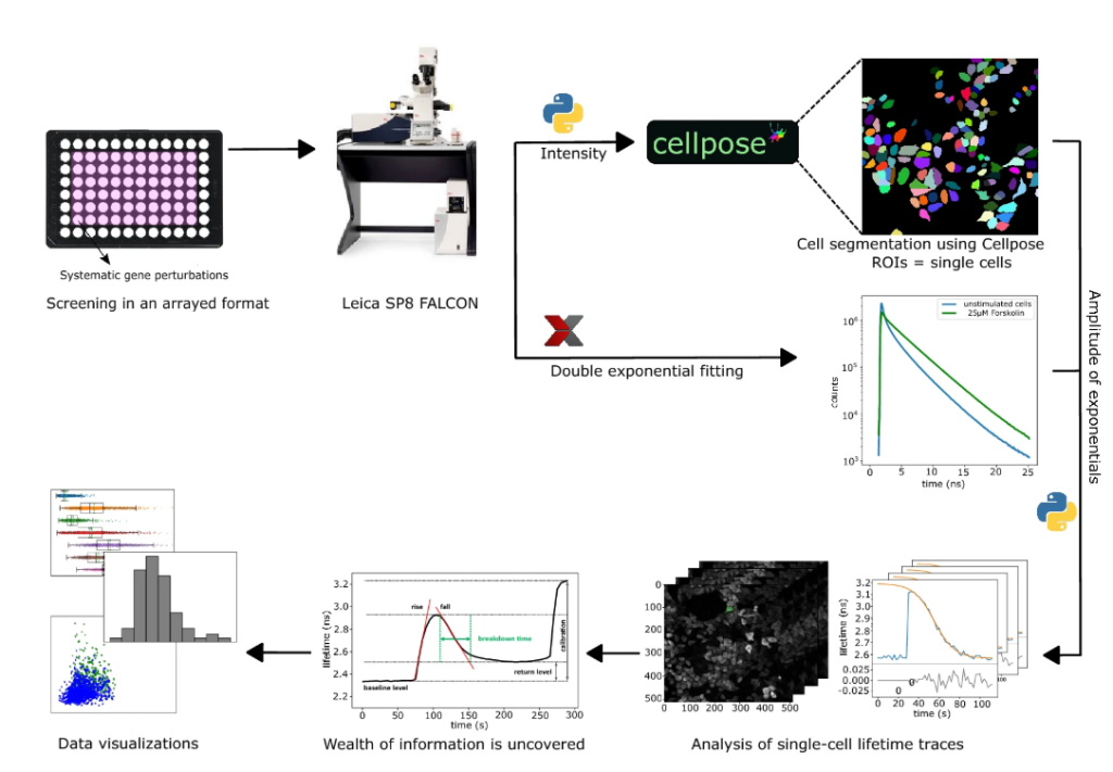
As mentioned previously, we chose a cAMP biosensor optimized for FLIM analysis. It has the advantage of featuring a tandem dark (non-emitting) Venus acceptor which allows recording a large part of the donor emission spectrum while minimizing contamination of the signal with acceptor emission8. The high FRET span and photostability of the sensor made it ideal for rapid screening purposes when the photon budget is limited. The screen was performed on the Leica SP8 FALCON system where we optimized the settings to collect large numbers of photons such that the S/N ratio of lifetime measurements is high while avoiding unnecessary photodamage. Experiments were conducted in 96-Well plates, imaging a FOV with ~200-600 cells per well, at 2 or 5 second time-lapse rate. One entire screen (imaging ~50 wells) took 6-8hours to complete – which was acceptable as it minimized the risk that factors like medium aging and change in cell confluency would influence our results. The stimuli (agonist + antagonist) were added manually to each well. In the beginning, we intended to automate this as well and had developed an Arduino-operated motorized pipetting system (see video). However, automated pipetting did not seem optimal for getting fast and reliable responses following stimuli addition. More details of our imaging settings and how the screen was performed has been outlined in the Methods section of our paper.
Next step after performing the screens was to fit and export the data for further analysis of the lifetimes.
Fitting the lifetimes:
We tested fitting our lifetime data in various manners. The photon arrival times recorded, showed a multi-exponential decay – which indicated an overlap of different FRET states. A double-exponential or 2-component fit described our data well, with a high FRET state with a low lifetime of 0.6 ns and a low FRET state with a high lifetime of 3.4 ns. After fitting, we saved two TIF files with the amplitudes of these two components, also reducing raw-data size by many fold. We then mapped the ratio of the components back to the original 0.6-3.4ns scale, resulting in a weighted mean lifetime value (to relate to conventional reporting system of lifetime values).
We report mean lifetime values calculated from two-components instead of using FALCONs mean photon arrival time (or single component fit), because using the latter proved to be quite sensitive to the environmental background light. Additionally, results with the 2-component fit had less pixel to pixel variation compared to a single component fit.
Automated analysis pipeline(AAP) & the pandemic
We next set out to develop the analysis pipeline. Believe it or not, but after the first screen, we extracted lifetime data from individual cells by manually drawing ROIs around ~ 5000 cells, followed by using 2 separate MATLAB scripts to analyze the lifetime data, calculate the breakdown time and data visualization! From that to our current automated analysis pipeline has been a very interesting journey.
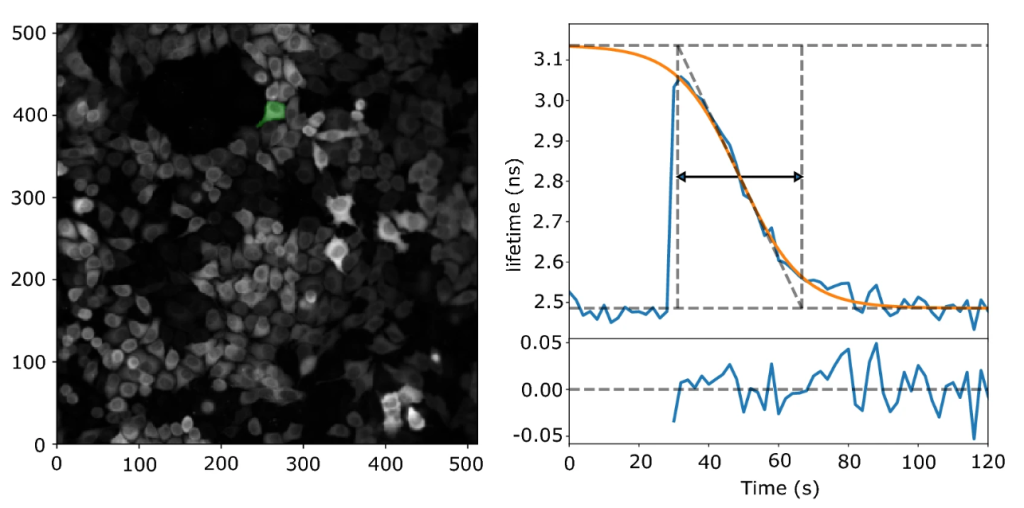
First, we implemented automated segmentation to extract lifetimes from single cells. For that we used Voronoi based segmentation, which segments cells based on nuclear staining. Output files were imported to MATLAB to analyze the lifetime data over the time course for single cells, fit them to a logistic function and extract various fit parameters – one of which was cAMP breakdown time.
The series of events that happened next only helped us in making our AAP much better than what it currently was: in mid-February 2020, the pre-print of Cellpose9 was published and in mid-March 2020 the Covid-19 pandemic hit us. Cellpose is a deep learning-based cell segmentation algorithm and upon seeing their pre-print, we had to try it out on our screen dataset. In comparison to our Voronoi based segmentation, Cellpose did not depend on nuclear staining and performed slightly better, although it took much longer. But since time was not a constraint, we chose to go ahead with Cellpose. However, Cellpose at that time was not compatible with Fiji and therefore, we decided to move to Python.
Around about this time, the pandemic worsened and going in-person to the lab stopped. Luckily, we were almost done with the majority of the experimental work (reproducing our observations, experiment repeats etc.), so it was the analysis pipeline that was left to develop. This gave us the time to shift our analysis pipeline to Python. “Work from home” largely boosted our lab members’ Python coding skills and finally we had a single pipeline for the entire analysis. This made it much simpler and more user-friendly, and it did not rely on close-source software anymore.
Significant challenges came our way when shifting from one programming environment to another, but when it was finally ready, we had added some new features to it as well! For example, we made a feature called “error traces” which served as a quality check for the traces to be included in the analysis (e.g. – error conditions such as disturbances by dislodged cells and out-of-boundary conditions). Programming this feature really tested our patience as one had to execute the code several times to make sure that the criterions weren’t too liberal or strict. Another feature we added was the “Results browser” which let us browse through individual traces, cell by cell. The results browser highlights the cell of interest and displays the corresponding trace while also listing key parameters such as goodness of fit and possible error conditions that were registered during analysis. Finally, with a fully functional pipeline it took us 3 hours to analyse 6 screens, with the cell segmentation consuming most of the time (N.B – Cellpose analysis can be almost 3 times faster if a CUDA enabled GPU is used instead of a CPU). After that, it was time to scrutinize our data – the part of the project that took most time to finish.
Scrutinizing the data:
Of course, we knew the most important result of our screen – PDE3A and PDE10A stood out as being the dominant PDEs in HeLa cells that regulate cAMP breakdown. However, we had to run multiple checks on our dataset in order to be confident about our interpretation.
We looked for hidden correlations, actual phenotypical and morphological differences between different traces and cells on different days. We checked whether the baseline lifetimes and thus cAMP levels were stable for the duration of the screen and found near-identical lifetimes in the experiments recorded at the onset and at the end of the 6-hour long screen. We also noticed that in the uncaging assay, PDE3A and 10A knockdown cells stand out even before photo uncaging, because the baseline levels in these wells were somewhat elevated compared to the other wells. So, in a way, the caged cAMP “leakiness” confirmed our results. However, since we sought to isolate the kinetics of cAMP breakdown, imaging cAMP breakdown after photo release was the most reliable way to find the “hit-PDEs” in HeLa cells. Most of these important checks made it to the supplementary information of our paper. However, few other things did not make it to the final cut – for e.g.: we also analyzed the data without fitting the decay. For this we took the response peak and extracted the time between 50% of the maximal response up to 50% of the return of the response (i.e., cutting off the top half of the peak and measuring its width). The results of this analysis were in excellent agreement with the fitting data but were left out in the final version of our paper.
Presenting our findings in a few conferences also led us into newer and deeper discussions about our data and analysis techniques with the scientific community. Finally, after multiple rounds of scrutiny and discussions, we were confident of our results. Adding a few more months to draft the manuscript and put everything together, we were ready to submit the paper to the journal and to post as a pre-print.
Final words and what lies ahead :
The writing and re-writing and scrutinization of the paper took a significant amount of time. If labs wouldn’t have shut down due to Covid-19, we had hopes of performing the screen on other cell lines as well to see if we identify different PDEs. This work will now still be performed and is reserved for a student-project in the lab.
All in all, we were content that with this new screening technique for dynamic phenotypes we had picked two hits very reliably. However, the biggest challenge that we faced throughout the project was cellular heterogeneity. We often saw varied responses of cells from day-to-day, making it difficult to get reliable results. Only when we had accumulated reproducible data from two lab members performing the screens on different days with different batches of cells, following two experimental protocols, we were confident about our results. This only enhances the point that cellular heterogeneity plays a big role when studying cellular responses at the single-cell level and extra care needs to be taken especially when performing screens. Another point that this project highlights is the importance of pre-prints. It took 9 months before Cellpose was finally published in Nature Methods (after being posted on bioRxiv), but by then we had already made significant progress in our work because of that pre-print. Even when we submitted our work as a pre-print for the first time, we were happy with the reaction and feedback our paper got from the community.
Looking ahead, we are preparing to apply “dynamic screening” in a pooled format instead of arrayed. As exciting as it sounds, it deals with a lot more technical challenges, however the throughput of a pooled screen is also higher!
– Written by Sravasti Mukherjee and Olga Kukk
References:
1. Esposito, A., Dohm, C. P., Bähr, M. & Wouters, F. S. Unsupervised Fluorescence Lifetime Imaging Microscopy for High Content and High Throughput Screening *. Mol. Cell. Proteomics 6, 1446–1454 (2007).
2. Padilla-Parra, S., Audugé, N., Coppey-Moisan, M. & Tramier, M. Quantitative FRET Analysis by Fast Acquisition Time Domain FLIM at High Spatial Resolution in Living Cells. Biophys. J. 95, 2976–2988 (2008).
3. Margineanu, A. et al. Screening for protein-protein interactions using Förster resonance energy transfer (FRET) and fluorescence lifetime imaging microscopy (FLIM). Sci. Rep. 6, 28186 (2016)
4. Luis A. J. Alvarez, Bernd Widzgowski, Giulia Ossato, Bram van den Broek, Kees Jalink, Lioba Kuschel, M. Julia Roberti, Frank Hecht. SP8 FALCON: a novel concept in fluorescence lifetime imaging enabling video-rate confocal FLIM. Nat. Methods 16, (2019).
5. Levitt, J. A. et al. Quantitative real-time imaging of intracellular FRET biosensor dynamics using rapid multi-beam confocal FLIM. Sci. Rep. 10, 5146 (2020)
6. Raspe, M. et al. siFLIM: single-image frequency-domain FLIM provides fast and photon-efficient lifetime data. Nat. Methods 13, 501–504 (2016).
7. Klarenbeek, J. B., Goedhart, J., Hink, M. A., Gadella, T. W. J. & Jalink, K. A mTurquoise-Based cAMP Sensor for Both FLIM and Ratiometric Read-Out Has Improved Dynamic Range. PLoS ONE 6, (2011).
8. Klarenbeek, J., Goedhart, J., van Batenburg, A., Groenewald, D. & Jalink, K. Fourth-Generation Epac-Based FRET Sensors for cAMP Feature Exceptional Brightness, Photostability and Dynamic Range: Characterization of Dedicated Sensors for FLIM, for Ratiometry and with High Affinity. PLoS ONE 10, (2015).
9. Stringer, C., Wang, T., Michaelos, M. & Pachitariu, M. Cellpose: a generalist algorithm for cellular segmentation. Nat. Methods 18, 100–106 (2021).
 (No Ratings Yet)
Get involved
Create an account or log in to post your story on FocalPlane.
More posts like this


Filter by
- NewsApply
- DiscussionsApply
- How toApply
- ToolsApply
- Case studiesApply
- InterviewsApply
- JobsApply
- EducationApply
- Blog seriesApply
- GloBIAS – updates fr..om the communityApply
- WAMBIAN: West Africa.. in FocusApply
- Volume EMApply
- Latin American Micro..scopistsApply
- Bio-image Analysis w..ith NapariApply
- Imaging with…Apply
- Towards Global Acces..sApply
- Latin America Bioima..gingApply
- From Zero to Qupath ..HeroApply
- Asian Microscopists ..and Cell BiologistsApply
- AIC at HHMI JaneliaApply
- Deep Learning for Bi..o-image analysisApply
- Highlights from Euro..-BioImagingApply
- LSFM seriesApply
- DIY MicroscopyApply
- View all