LSFM series – Part III: Image acquisition: Calibration and acquisition
Posted by Elisabeth Kugler, on 17 December 2020
Elisabeth Kugler 1 and Emmanuel G. Reynaud 2
Contact:kugler.elisabeth@gmail.com; emmanuel.reynaud@ucd.ie
Now, we are getting closer to the point of setting up our sample in the chamber to image it. Now that we know which microscope we are about to use (Part I) and have mounted it the right way (Part II), we need to trust it! For some this might mean: “As long as it starts, we will be fine!”. No, is the short answer and we will explain why below. So, brace yourself for a boring but essential checklist to get a match, like made in heaven, between your sample and the imaging system.
1. Lasers do die!
Yes, your first second-hand car was OK to get you from A to B in slow motion but between the rattling of the air conditioning and the strange noise letting you know that you are somewhere between the first and second gear, this was definitively an untrustworthy ride. So, what about your microscope? Start. If you want the best out of this piece of machinery, then you need to be able to check its capacities as lasers do die! Intensity will decrease and affect exposure time, which could be detrimental for quantitative measurements over a couple of years of imaging. Similarly, stages and other optical components will decrease in performance over time, especially when used by different users.
The best solution is calibration! As a reminder, in light sheet fluorescence microscopy it is essential that the illumination plane is perfectly aligned with the detection focal plane (Fig. 1A). The typical protocol for optical system calibration is the use of fluorescent beads. As they are well-defined points, they can be easily seen and allow for the measurement of the almighty Point Spread Function (PSF), the parameter that defines how an optical system convolves a point into something rather “spread”. This can be a handy parameter for later deconvolution of your data. In LSFM, beads also allow you to check that you are in focus across field of views (FOVs). If you can perform or learn to perform this calibration step it is a plus, but often commercial systems will have established a protocol to do so. Do it regularly and keep a record of this step in your experiment folder as it can be useful to trouble-shoot issues later. A well-tuned microscope will always deliver better data (Fig. 1B-D). Familiarize yourself with the important parameters of your favourite scope and keep track of them, as they are as valuable as the sample you use and the antibody stain you perform. At the end of the day, you analyse the images not the sample.
2. Acquisition protocols
Ready! The sample is in the FOV and you have chosen the perfect angle to start recording. Steady! Have you all the right information? It is always a good idea to plan your acquisition protocol(s) in advance.
The sample: If working with a sample you are not that familiar with it is key to examine your systems capacities to work with it. Is the sample well mounted and well labelled? A quick check under a widefield fluorescence microscope or a binocular may save you time and efforts. Do not chance it, check it!
The gears: Is it the right objective (air/water/oil; numerical aperture (NA); magnification), did you rightly combine the illumination objective with the detection objective, producing the right amount of magnification, FOV (Fig. 1E, F), and light sheet thickness? What depth of field can you achieve and to which point does it make sense (Part I)? Are you using digital (cropping with reduced resolution) or optical (enlarges the images, while keeping resolution) zoom? In a multi users’ environment, things can change quickly at the microscope, such as dirty fingers, different settings, or unplugged equipment. A quick run-through, which follows the flow from power source to microscope, laser/LED, objectives, camera, stages and finally the imaging software will make sure that things are the way they are meant to be.
Time-lapses: Is your FOV appropriate to allow image acquisition even with sample motion and growth (e.g. if imaging 24 hours, how large will your sample be at the end)? When you image over time, your set up should accommodate the endpoint (e.g. growth and pigmentation) from the start not the inverse and do not forget to leave some 10 to 20% margins. It also means that you should check the data as soon as possible. If something went wrong during your time-lapse, do the right thing: DELETE!
Your lasers and signal: Have you checked that you are using the optimum trade-off between laser power, exposure time/gain, and offset? If imaging time-lapses, have you considered how your reporter will behave over time (brighter, dimmer?) and noise (especially scattering and auto-fluorescence)?
Imaging multiple fluorophores: Are you separating the tracks sensibly (e.g. spectral overlap and filter systems)? Which one are you imaging first (e.g. excitation bleed through (or crossover or crosstalk) often happens in the blue spectrum; emission bleed through often happens in the red spectrum)? Are the tracks aligned (e.g. if something should truly overlap, does it)?
Even though the above seem extensive and you may be a bit confused or even totally lost, don’t panic, most of these aspects are learned over time and pilot experiments are crucial to learn what works and what simply does not. Will you buy randomly a car online no question asked? Or a test drive is on the agenda? Get through the list step-by-step and learn along the way. Knowing how to image correctly and learning the ropes will give you confidence in your data and improve reproducibility. Keeping records and notes on the above is key to optimizing the setup for best image quality, extending imaging duration, ensuring consistency between experiments, as well as training new users.
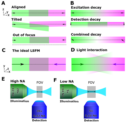
Figure 1. Know your system. (A) The illumination path (green and magenta) should be aligned with the objective focal plane (dotted line). (B) As discussed in Part II, the system suffers from decay in the excitation and emission plane. (C, D) Even with “perfect” calibration, light interaction with matter interferes with imaging. (E, F) Know your FOV and how it is affected by your imaging setup.
3. Light sheet thickness and variable resolution
Many of us are often obsessed with the holy “Resolution” and want the best out of data. The general concept in LSFM relies on the light sheet, the detection plane, and how they overlap; often summarized as “the light sheet thickness”, which allows the scope to “slice” the sample space optically. For many, it is translated as “the thinner the slice, the better the resolution”. This is partially true, and you will find in the reference section a paper that will sort this out for you. In summary, slicing an elephant at 50µm is useless if you want to count the number of legs. Also more slices, more data, more acquisition time, more laser power and so on…a very slippery slope (Part IV)! You must adapt your sampling frequency to your sample and biological question, making it the most sensible as it will directly affect your image processing and extracted results. Oversampling is wasted effort and time and disk space.
LSFM is seen as a 3D imaging technique and so the resolution has been considered in lateral and axial directions. Confocal, for example, typically has a better lateral than axial resolution. It is the same for LSFM, but the optical sectioning is better due to the light sheet, thus the axial resolution as well as depth of field is better than with confocal, depending on the system of course. However, it is still an optical imaging technique and as we discussed before (Part II) the deeper the light sheet goes and the deeper you image the worst both resolutions will get. The typical problem is wanting to image the entire sample, even if not entirely necessary. This will result in uneven resolutions across the sample, especially in large or scattering samples, creating a nightmare for deconvolution and other image processing steps that will follow. In this case more data is definitively not better. Be smart, learn to assess resolution decay and set up limits to limit data collection while improving resolution across your data and image processing,
So why does all this matter?
When talking about microscopy, we often say “seeing is believing”. However, relying on images, we need to be confident to know how these where produced and that the images are free of artefacts in imaging or analysis. One of the most common errors is that users forget the difference between axial and lateral resolution, assuming that their voxels and data are isotropic (i.e. a voxel is the same size in x, y, and z direction). Pixels are by definition and physically a perfect square on the camera chip while they are actually a point. The voxel, on the other hand, is defined by the pixel size as well as the z-axis sampling (i.e.slice thickness). In fact, voxels are longer in the z-axis, due to reduced resolution. When applying 3D analysis steps this might lead to false quantification outputs if voxels are anisotropic, and some workflows do not work at all due to being developed for medical imaging, which generally produces isotropic data.
Thus, whatever data you produce, before processing it is advisable to look at your image properties using these simple steps (we have learned these things the hard way!):
- Check your pixel ratio (x, y).
- Check properties of voxel size: is x, y, z information existing and in what unit?
- Check image properties to check that metadata are correct: e.g. is information on slices and time stored correctly.
- Check after the individual processing steps that the above information is preserved.
- Use 3D rendering to look at your data (we have seen “squashed” data way too often), to understand spatial relationships and how voxel size impacts these.
Together, it becomes clear that the more you know about your system, the better you understand your data and image analysis needs.
May the LISH be with you,
Elisabeth and Emmanuel
P.S.: If you want to share your views, do not hesitate to get in touch.
Associations / Institutes
(1) Institute of Ophthalmology, Faculty of Brain Sciences, University College London, 11-43 Bath Street, LondonEC1V 9EL. (2) School of Biomolecular and Biomedical Science, University College Dublin, Belfield, Dublin 4. Ireland.
Acknowledgements
We are extremely grateful to Johannes Girstmair and Rob Wilkinson for their constructive feedback!
Further Reading
- Elena Remacha, Lars Friedrich, Julien Vermot, and Florian O. Fahrbach, (2020) How to define and optimize axial resolution in light-sheet microscopy: a simulation-based approach, Biomed. Opt. Express 11, 8-26
- Anna Payne-Tobin Jost, Jennifer C. Waters (2019); Designing a rigorous microscopy experiment: Validating methods and avoiding bias. J Cell Biol 6 May 2019; 218 (5): 1452–1466.
- Power RM, Huisken J. (2017) A guide to light-sheet fluorescence microscopy for multiscale imaging. Nat Methods. 2017 Mar 31;14(4):360-373.
 (No Ratings Yet)
Get involved
Create an account or log in to post your story on FocalPlane.
More posts like this


Filter by
- NewsApply
- DiscussionsApply
- How toApply
- ToolsApply
- Case studiesApply
- InterviewsApply
- JobsApply
- EducationApply
- Blog seriesApply
- Latin American Micro..scopistsApply
- Bio-image Analysis w..ith NapariApply
- Imaging with…Apply
- Towards Global Acces..sApply
- Latin America Bioima..gingApply
- From Zero to Qupath ..HeroApply
- Asian Microscopists ..and Cell BiologistsApply
- AIC at HHMI JaneliaApply
- Deep Learning for Bi..o-image analysisApply
- GloBIAS – updates fr..om the communityApply
- WAMBIAN: West Africa.. in FocusApply
- Volume EMApply
- Highlights from Euro..-BioImagingApply
- LSFM seriesApply
- DIY MicroscopyApply
- View all