Rescaling images and pixel (an)isotropy

This blog post shows the importance of rescaling 3D image data and what anisotropy of pixels/voxels has to do with it. We will see which different options exist to rescale an image as well as their advantages and limitations. We will also apply a commonly used segmentation algorithm, Voronoi-Otsu-Labeling, on the original and the rescaled data to see the difference.

Voxel isotropy as a precondition for many algorithms

During Image Acquisition, physical limitations and the configuration of the microscope typically lead to a different voxel size in x and y compared to z. The voxels are anisotropic. However, some filtering and segmentation algorithms, like Voronoi-Otsu-Labeling, and also quantitative measurement methods may have isotropic voxel size as precondition. If these preconditions are violated, the results can be misleading or even wrong.
For this reason, the proper scaling of your 3D dataset is an important preprocessing step for the development of your image analysis workflow.

Often you can already see that your voxels are anisotropic when opening your dataset. In this blog post we will explore a dataset from Ozpolat, B. et al licensed CC BY 4.0.

It shows cells with marked membranes and nuclei of the marine annelid Platynereis dumerilii, but here we only use a single channel.
For image visualization and scaling, we use napari in this blog post.

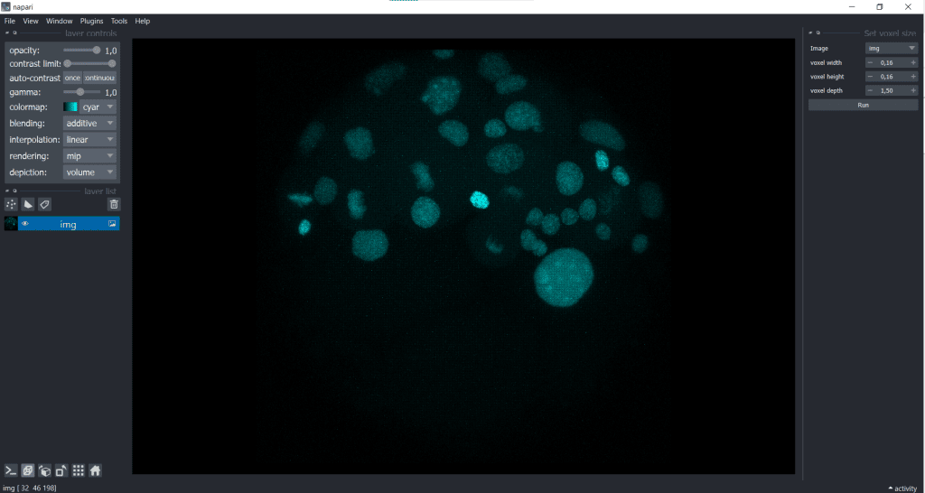
x-y-plane	y-z-plane

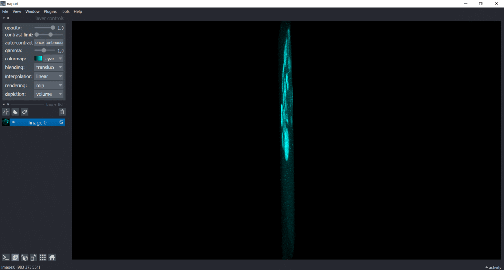In the image on the right, the y-z-plane is visualised but in a squeezed way.

Note: You can follow the demonstrated workflow in the related jupyter notebook here.

The voxel size of the image data is

voxelsize_x = 0.1596665040315075
voxelsize_y = 0.1596665040315075
voxelsize_z = 1.5

This information was derived from the czi-file and can also be found in our jupyter notebook.

As you can see, the voxels are nearly 10x bigger in z than in x & y.

Requirements

In this blogpost the following napari-plugins are used/mentioned:

• napari-layer-details-display
• napari-pyclesperanto-assistant
• napari-segment-blobs-and-things-with-membranes

Note: I would recommend to install devbio-napari. It is a collection of Python libraries and Napari plugins maintained by the BiAPoL team, that are useful for processing fluorescent microscopy image data. It contains all of the mentioned napari-plugins. If you need help with the installation, check out this blogpost.

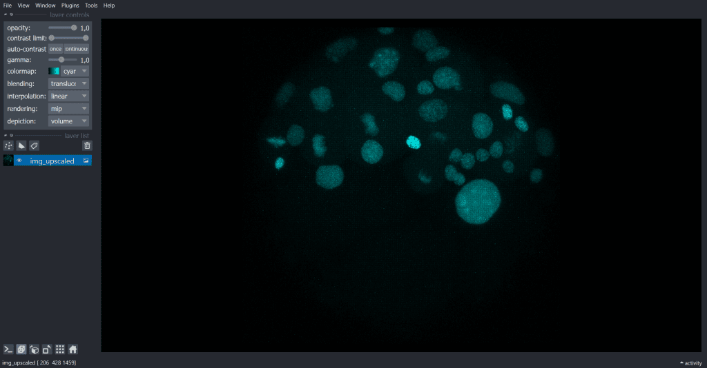
Layer Details and Visualisation adjustment in napari

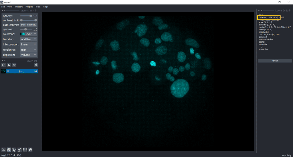
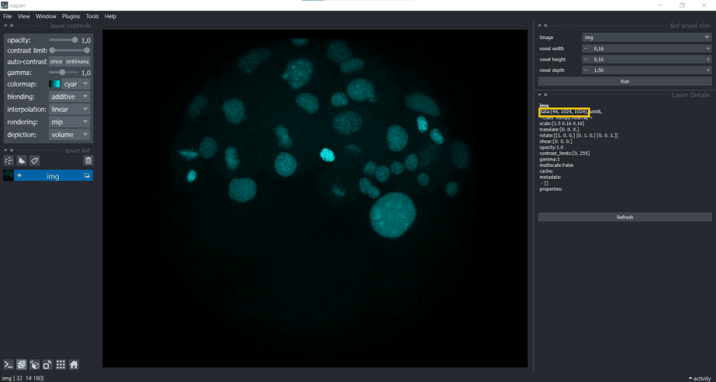
We can see our image shape when going to Tools/Utilities and selecting Layer Details:

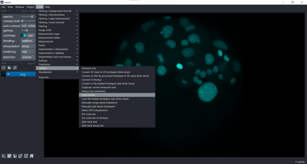
In this case, our image shape is displayed in the top right corner

We can easily fix the visualization by going to Tools/Utilities selecting Set_voxel size like this:

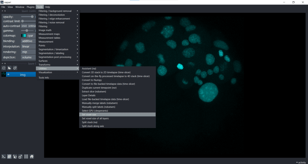
and then typing in the voxel size in x, y and z:

We receive the following change in displaying of our data:

x-y-plane	y-z-plane

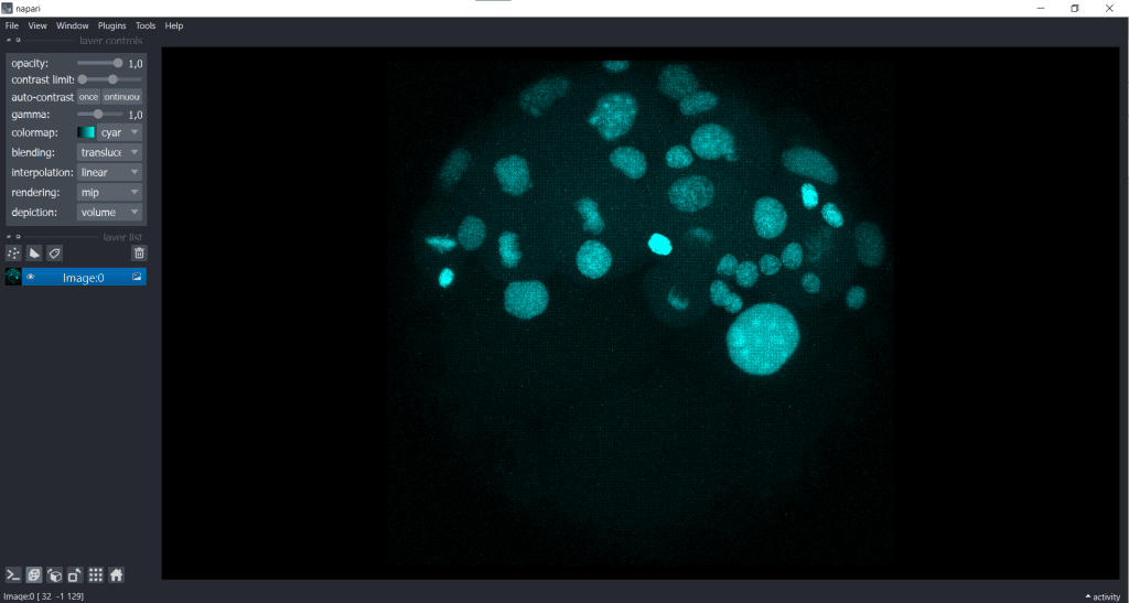Hereby, we only modified the visualisation and did not actually adjust the voxel sizes. The image has still the same shape which we can check again in Layer Details:

In fact, if you open a proprietary image file using a napari-plugin, like napari-aicsimageio, this change of displaying is often already automatically applied.

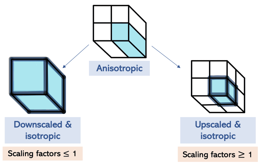
When we rescale the image, we are also changing the image shape and we can do this by down- or upscaling.

The difference between down- and upscaling

During downscaling, information is reduced and the image shape is reduced, whereas during upscaling new voxels interpolated from the existing ones are added to reconstruct the image. Hereby no new information is created, but the image shape is increased.

For down- and upscaling, we need to use scaling factors.

Scaling in napari using clesperanto

We will see in this section one example of scaling in napari using clesperanto. In the jupyter notebook you can also see other possible ways.

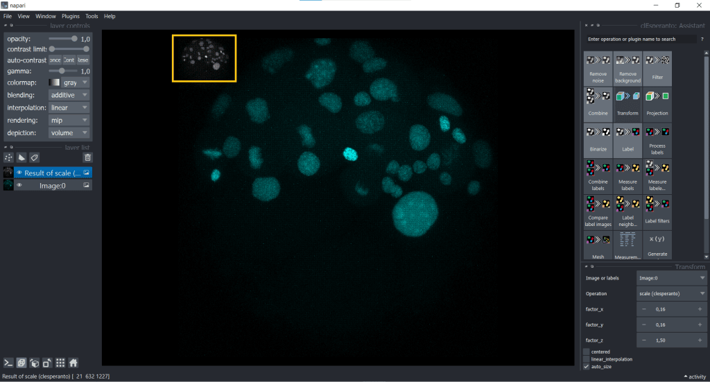
First, we open under Plugins the clEsperanto: Assistant. Now you can find under Transform the clesperanto–scale function

Scaling using the image voxel size

First, we have a look at rescaling using the image voxel size.Here, we are doing both down- and upscaling at the same time: downscaling in x and y (voxelsize < 1), while upscaling in z (voxelsize > 1)

The rescaled image looks like this:

x-y-plane	y-z-plane

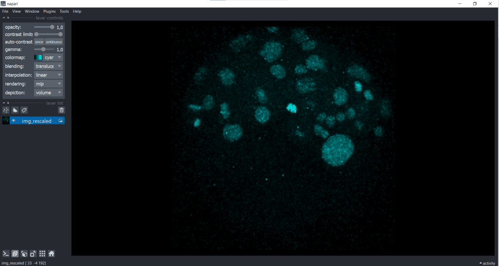Basically, you can see that rescaling leads to an adjustment of the image to better fit the size of the object being observed. Nevertheless, during rescaling using the voxel size, there is an information loss because of the downscaling in x and y.

To illustrate this information loss better, you can see here one slice of the dataset (2D) which was rescaled with the following scaling factors

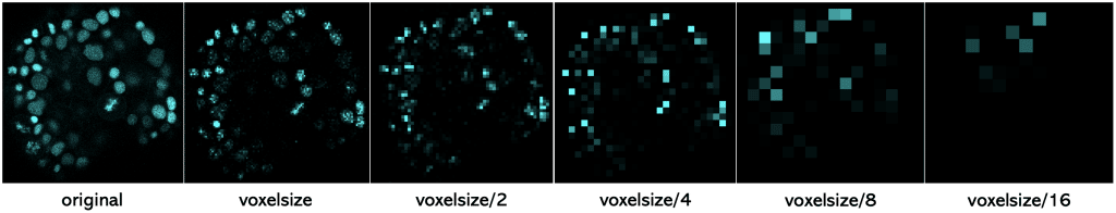
To sum this up, if you scale an image with its voxel size, the resulting image has a voxel size of 1 (µm). And if you scale an image with voxel size/2, the resulting image will have a voxel size of 2 (µm). And with larger voxel size, we loose more and more information.

Upscaling

If we don’t want to loose any information, we can also upscale our image. One reasonable idea would be using the voxel size of x & y as a reference like this:

• scaling_x = x/x = 1

• scaling_y = y/x = 1

• scaling_z = z/x = 9.43

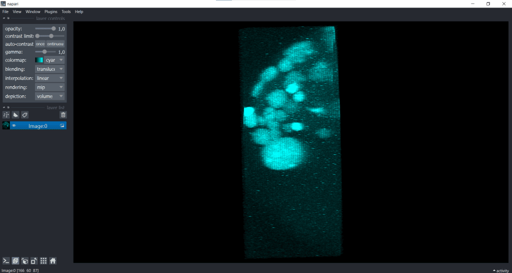
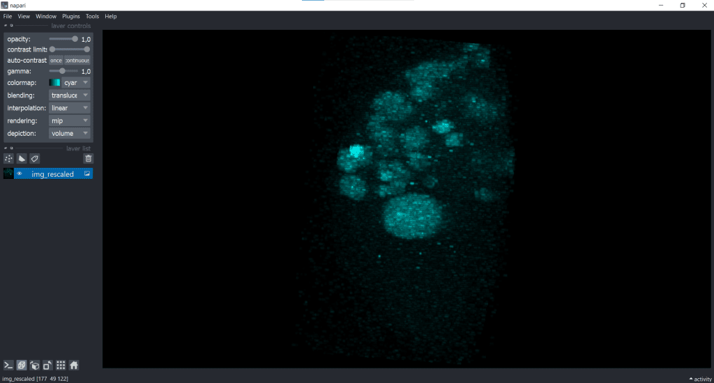
The result looks like this:

x-y-plane	y-z-plane

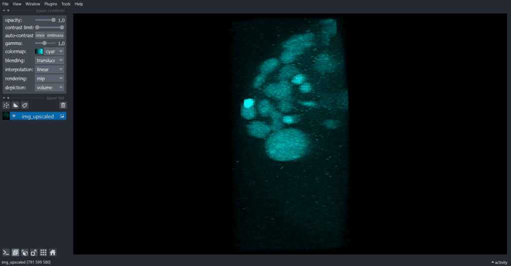Demonstration of how anisotropic voxels can manipulate measurements

As already mentioned, some algorithms need isotropic voxels in order to perform correctly. One example of a segmentation algorithm is Voronoi-Otsu-Labeling. Now we will investigate which time is needed to apply Voronoi-Otsu-Labeling on the anisotropic, the voxel size-scaled and the upscaled image and look at differences of the output.

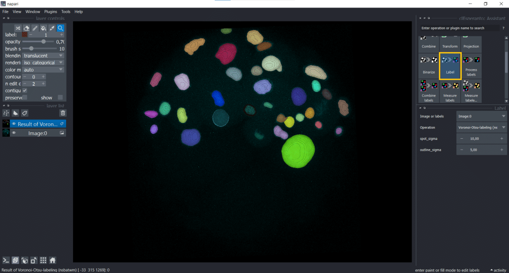
Voronoi-Otsu-Labeling

We select under Label Voronoi-Otsu-labeling(nsbatwm) and can now modify the spot_sigma and the outline_sigma. I chose spot_sigma = 10 and outline_sigma = 5 (the unit for this library is voxels):

And depending on if we apply this algorithm to the anisotropic, the voxel size-scaled and the upscaled image, the time differs:

Image	Time for Voronoi-Otsu-Labeling [in seconds]
Anisotropic	13
Rescaled using voxel size	0.4
Upscaled	144

You can see why upscaling can lead to memory and storage problems and why downscaling is the more often used method.

Now lets have a look on the segmentation result of the anisotropic and the upscaled image:

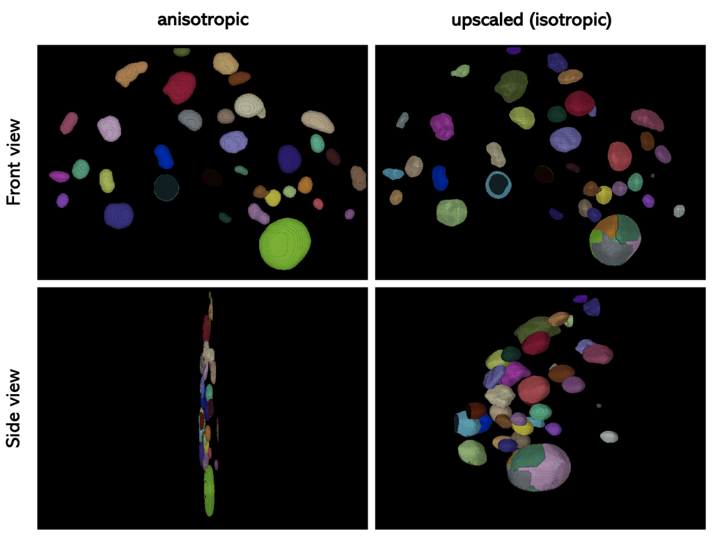
If we compare the result of Voronoi-Otsu-Labeling on the anisotropic and the upscaled image, we can see that the scaling has an influence on the performance of the algorithm.

Summary

In summary, when choosing between up- and downscaling there are advantages and limitations to both of them:

scaling	down	up
advantage	faster, less storage needed	no information lost
disadvantage	information is reduced which could be important, less details visible (which are maybe not needed for cell segmentation anyway),	the amount of information does not increase through interpolation, slower, might not fit into RAM or GPU memory

Which one to choose depends on the individual usecase.

Feedback welcome

Some of the napari-plugins used above aim to make intuitive tools available which are commonly used by bioinformaticians and Python developers. Moreover, the idea is to make those accessible to people who are no hardcore-coders, but want to dive deeper into Bio-image Analysis. Therefore, the feedback from the community is important for the development and improvement of these tools. Hence, if there are questions or feature requests using the above explained tools, please comment below, in the related github-repo or open a thread on image.sc. Thank you!

Acknowledgements

I want to thank Dr. Robert Haase as the developer behind the tools shown in this blogpost. This project has been made possible by grant number 2022-252520 from the Chan Zuckerberg Initiative  DAF, an advised fund of the Silicon Valley Community Foundation. This project was supported by the Deutsche Forschungsgemeinschaft under Germany’s Excellence Strategy – EXC2068 – Cluster of Excellence “Physics of Life” of TU Dresden. 

Reusing this material

This blog post is open-access, figures and text can be rused under the terms of the CC BY 4.0 license unless mentioned otherwise.

(5 votes, average: 1.00 out of 1)