Analyzing calcium imaging data using Python

Andrey Andreev
California Institute of Technology, David Prober lab
aandreev@caltech.edu

Calcium imaging allows tracking neural activity in time with single-cell resolution. There are many questions you might be interested in answering using this technique: which cells are tuned to the stimuli? is there periodic activity present in the data? which cells act together? how complex is the activity pattern? how many connected communities are present across the brain recording?

Previously we discussed initial steps for presentation of calcium imaging data. Here we continue offering example solutions to data analysis in the form of python notebooks bundled together with sample zebrafish Tg(HuC:GCaMP6s) data, acquired using 2-photon light sheet microscopy. We hope that these notebooks will serve as a springboard for people new to data processing and display using jupyter. All notebooks and data can be accessed through CaltechDATA doi.org/10.22002/z1m2d-jgm12. We present examples of the following analysis:

1. Analyzing periodic activity using periodogram
2. Resolving different sampling rate of neural data and stimuli data using interpolation
3. Application of Principle and Independent Components Analysis to calcium imaging data with scikit-learn
4. Representing neurons as network for graph theory analysis using NetworkX

Analyzing periodic activity

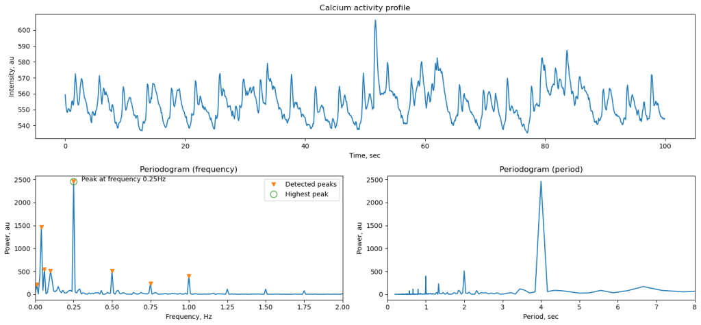
Periodic activity is present in brain of various model systems, including mice, zebrafish, and organoids [ref]. To quantify it, we use spectrum analysis often implemented using Fourier transform that decomposes initial data into sum of periodic signals. Amplitude of each signal can be extracted to analyze what is the dominating frequency of oscillations in the data. Conveniently, Sci-Kit library allows such analysis using periodogram function. Here we look at temporal dynamics, so spectral data can be presented in frequency domain (measured in Hz) or period (seconds). In this example, we apply periodogram to a GCaMP signal from zebrafish optic tectum, when sinusoidal light stimulation is present. Calcium signal generally follows tightly the stimuli oscillations, which results in very sharp peak in the frequency plot.

The duration of the recording and the resolution are tightly linked. Longer recording will provide proportionally higher spectral resolution and ability to distinguish closer frequencies if more than one present in data. However, biological data is noisy and longer recording can also cause broadening of the spectral peak through accumulation of variability.

ax1.set_title('Calcium response profile')

plt.plot(brain_data_ts, brain_data_int)
ax1.set_xlabel('Time, sec')
ax1.set_ylabel('Intensity, au')

ax2 = plt.subplot(223)
ax2.set_title('Periodogram (frequency)')
# extract time between frames from the first column in data
dt = brain_data[1,0] - brain_data[0,0]
print('Time between frames: ',dt,'sec')
fs = 1/dt # frequency in Hz

f, p = sc.periodogram(brain_data_int,fs)
plt.plot(f,p)
# find peaks:
peaks_locations, peaks_properties   = sc.find_peaks(p, prominence=200)

Full working notebooks and data are accessible via doi.org/10.22002/z1m2d-jgm12

Reconciling signals recorded at different rates

We often want to compare how closely the response follows the stimuli, for example, using Pearson’s correlation. In case when our stimulation signal data has higher temporal resolution (more data points per unit time) than the calcium recording, we need to apply interpolation and artificially increase sampling rate of the calcium data. In our example we have high-resolution (100Hz) signal that is driving light source, and much slower recording of the brain activity (10Hz). Interpolating brain signal to have same number of data points will allow us to use built-in function for correlation analysis.

# The brain and LED data are different size, so to reconcile we use interpolation
print('Brain data size: ', len(brain_data_ts)) # 1000 samples of brain activity data
print('LED data size:   ', len(stim_data_ts))  # 10000 samples of LED intensity data

brain_data_interpolated = np.interp(stim_data_ts, brain_data_ts, brain_data_int )
# brain_data_interpolated will contain values generated to fit the finer stim_data_ts time points
print('Brain data interpolated size: ', len(brain_data_interpolated)) # 10000

Using PCA and ICA with two-dimensional calcium imaging data

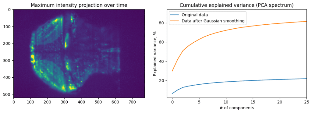
Calcium imaging data often contains a lot of pixels and time points, which is why we call such data “high-dimensional”. Using dimensionality reduction tools such as PCA allows compression of data and removal of background information. Use of Independent component analysis (ICA) allows extraction of dominant signals from the data and splitting it into primary components as we’ll show below. We use implementations of PCA and ICA in the scikit-learn package.

We will treat different neurons (or image pixels) as observations and time points as features. It can be difficult to jump from general discussion of PCA given in statistics class to application of this method to calcium imaging data. PCA can be understood using the following example: imagine we collect data about dogs, measuring their weight and height. Weight and height are variables (features), and each dog represents an observation (sample). In calcium imaging world, when applying PCA, each pixels represents variable, and each time point is an observation.

Cumulative explained variance plot shows how much of data variance is contained in the first N principal components. If the neural activity of all cells is highly correlated, then first principal component will explain most of the data. Data with more noise, or more heterogenous activity, will have slower accumulation of explained variance. We can see that by comparing PCA of original data and PCA of data blurred using spatial Gaussian filter.

Applying PCA, while treating each time point as a sample, and each pixel as feature, we can extract main component of activity. However, that is not enough to make meaningful conclusions about data, as PCA aims to pool together pixels containing the most amount of information. This will be necessity average a lot of different activity profiles. To decode finer details, we can apply Independent component analysis (ICA) after PCA dimensionality reduction. That is, first we will compress our data from 500×700 pixels to 20 principal components, and then apply ICA to these principal components to find four independent components that comprise most of the independent information.

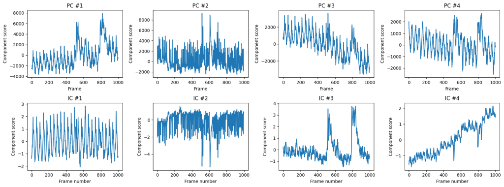
One of the application for ICA is removal of motion artifacts and other common-mode signals from the calcium imaging data (see Hanson et al, 2023). Here we see that IC #1 contains periodic activity, and IC #3 contains large-scale spikes. Together these components can be recombined into first principal components. We can see which pixels contribute to the first independent component:

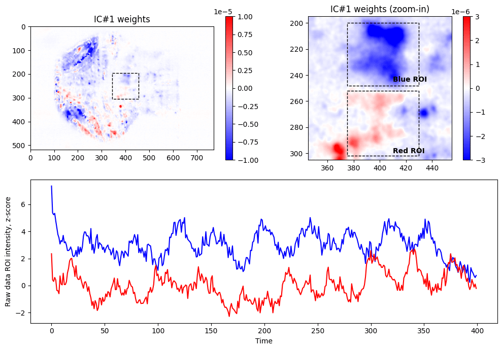
In order to generate image of weights for ICA (top left panel above), we need to perform matrix multiplication of weights of the PC components by the weights found through ICA, followed by reshaping of the resulting array to be represented as 2D image:

IC_2d = np.matmul( np.transpose(PCAmodel.components_[0:N_PCs, :]), ICAtransformer.components_[IC_i,:] )
IC_2d = np.reshape(IC_2d, (Ny,Nx))
plt.imshow( IC_2d ,cmap = 'bwr' , vmin=-1e-5, vmax = +1e-5)

Looking at the weights of first IC, we are noticing that there are two clusters (within dashed box), one with positive weights (red) and one with negative weights (blue) contributing to the IC #1. Zooming in and selecting approximate ROIs around these clusters we can extract raw fluorescence signals from the data (blue and red lines). As expected from seeing weights of different signs, these raw fluorescence traces are anti-correlated (Pearson’s R = –0.11, p<0.05).

r = pearsonr(blue_pxs_data, red_pxs_data)
print(f"Correlation between red and blue lines: %0.2f (pvalue = %0.2f)" % (r.statistic, r.pvalue))
# => Correlation between red and blue lines: -0.11 (pvalue = 0.02)

It is important to note that we went into that analysis without expecting seeing such clusters of activity, and final anti-correlated traces are extracted from raw fluorescence imaging data, and not in any other way processed. PCA and ICA allowed detection of pixels that have opposite activity pattern, and also located in areas studied previously to be responsible for vision (similar observations were reported previously in more sophisticated experimental paradigms, see Dunn et al, 2016 or Chen et al, 2018).

Network-level analysis of neural communities

Finally, we present application of NetworkX library to calcium imaging data. First step when constructing network (or graph) analysis, is deciding what constitutes a node (we pick individual pixels) and defining distance metric between nodes (we pick square of Pearson’s correlation). Using this metric we construct pairwise distance matrix that is the heart of the network analysis.

First, we select subset of pixels from the imaging data. We pick random set of pixels and then filter pixels that correlated with average movie intensity. That will avoid using background pixels or other pixels that don’t correspond to majority of activity.

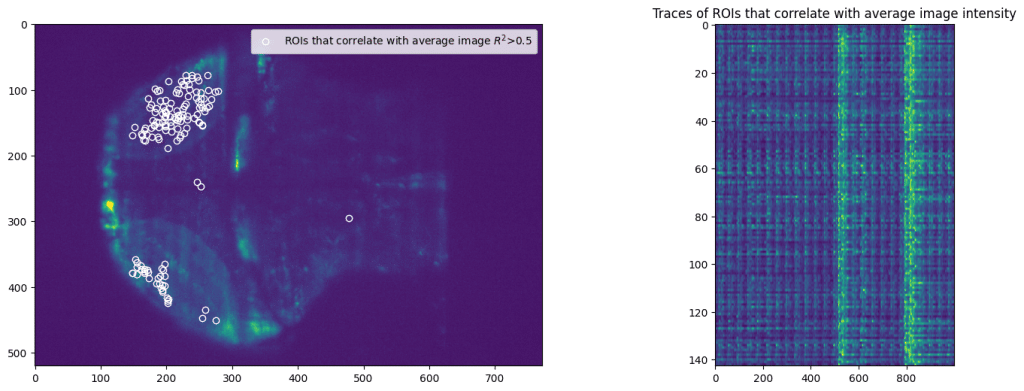
Application of NetworkX library allows easy access to multitude of analysis tools, from computing trophic levels of nodes to calculating current-flow betweenness centrality or finding an asteroidal triple in the graph. However, here we present an application of slightly more popular algorithm, namely finding communities within the graph. Communities are broadly characterized as groups of nodes that are more closely connected with each other than other nodes. Precise definitions of community depend of the specific details of given algorithm. Here we apply search for k-clique communities in neural activity data (see Kai Wu et al, 2011 for more details). After calculating correlation between all selected ROIs, we perform further pruning of the network and remove all “weak” edges with correlation Pearson’s R^2 < 0.7.

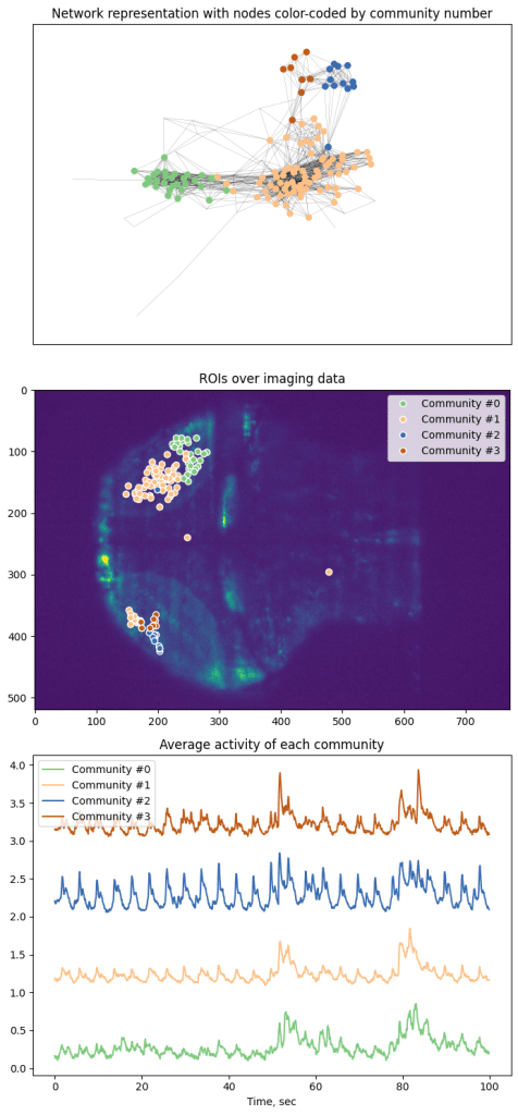
Here we represent every node as a point and color-code based on 6-clique communities. However, algorithm was able to only segment graph into 4 communities based on the data.

Conclusion

This article and associated data and Jupyter notebooks (doi.org/10.22002/z1m2d-jgm12) are released as a set of concrete example of analysis for calcium imaging data. In no way it was designed to be a full tutorial with ample explanation of algorithms and approaches. Reader are welcome to reach out to the author and use that document as a conversation started with their colleagues such as more knowledgeable software developers. Scripting of analysis and data presentation (that we discussed in previous article) is a necessity in modern research, especially data-heavy field such as microscopy, but learning new tools can be arduous. We hope that this article will encourage you and help on this journey.

(No Ratings Yet)