LSFM series – Surfing on the data freak wave! Part II: Before imaging: Know your sample (geometry)
Posted by Elisabeth Kugler, on 10 October 2020
Elisabeth Kugler 1 and Emmanuel G. Reynaud 2
Contact: kugler.elisabeth@gmail.com; emmanuel.reynaud@ucd.ie
In imaging, resolution is one thing, but the essential element is the sample, right? You want it all; the best spatial and temporal resolution and extracting juicy data by the Terabyte load. However, the ease and speed of data acquisition with LSFM is not always a good thing and bad data is trash data (e.g. DELETE). Defining “good data” is not straightforward, but we can agree that data with extensive signal artefacts, motion artefacts, the wrong angles, or with unsatisfying time intervals are not in this category. We want signal, not noise! Data quality is crucial for meaningful analysis, and in this time of climate change emergency, remember that also data have a carbon footprint. We here discuss how spending time on sample preparation and setting up your LSFM can improve data quality. Thus, how to avoid recording useless data.
Sample preparation
Each sample has its own geometry, its own temporal characteristics and its own physical features (e.g. transparency). Spending time on sample preparation will reduce the actual time required for data acquisition and increases comparability between imaged samples and ease of processing.
Rule one, if you want to fail miserably, rush to the microscope, failure guaranteed! Rule two, spend some quality time staging and sorting your samples before starting on the LSFM. When working with living animals, anaesthetics are often needed to induce a loss of physical sensation and movement. However, they can wear off with temperature, salinity, and light. Thus, using freshly-made or short-term stored anaesthetic is essential, especially if wanting to setup long-term time-lapse experiments.
Various setups for sample mounting exist (see Zeiss Z.1 user manual) and what is best for your data, depends on the LSFM you use (e.g. see Blog Part I), as well as your biological question. Each LSFM has a «sample space», typically a Lattice Light Sheet has a very tiny sample chamber, while mesoscopic systems have a swimming pool. Know the space you can use safely.
For all acquisitions, especially time-lapses, four main things need to be considered, namely: (a) mechanical stability, (b) minimal impact on the sample (eg. allows for development), (c) supports the sample and imaging (e.g. refractive index, geometry), and (d) acquisition optimization (see below).
The most commonly used approach for mounting is embedding. Here it is crucial to use agarose free of any debris, fully polymerized, and that the sample-to-agarose ratio is about 1/3-2/3. Agarose is not made for imaging so keep it clean, as a sterile product (e.g. hood), aliquoted and in the dark (e.g. oxidation). With too little agarose, mechanical stability can be compromised; too much, and lightsheet penetration can be affected with agarose chains absorbing in the UV range. Low melting point (LMP) agarose is particularly useful when working with temperature sensitive samples (melts at around 65°C; sets at about 30°C) and it can easily be aliquoted.
Light interacts with matter…the deeper the worse (applies to detection too…)
Light interaction with matter is particularly challenging in samples with a refractive index different to the imaging medium (e.g. non-transparent opaque samples) in which transmission, reflection, refraction, diffraction, absorption and scattering interfere with light rays (Fig. 1A-C). Additionally, non-linear interactions and artefacts (Fig. 1D) can occur in fluorescence microscopy. Similarly, structures, such as skin pigmentation or lipids in the yolk interfere with the light path. These alterations of beam paths can result in artefacts such as that nuclei in the middle of an object appear to be larger, but are not. Whatever your sample transparency, light will always be affected by matter. Thus, is the case for both, the illumination laser beam as well as emitted fluorescence photons.
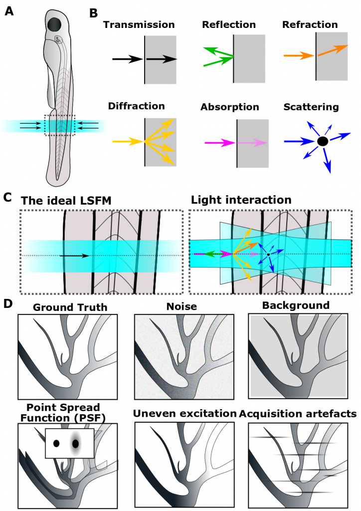
Figure 1: Light interacts with matter. (A-C) Light rays are impacted by refractive index changes.Ideally, light penetrates the sample undisturbed; however, light interaction with matter leads to beam path alterations. (D) Object features and imaging artefacts further contribute to non-ideal data acquisition.
In most LSFM, the imaging setup allows for free translational movement in 3D (x, y, z) as well as 360° rotation around the sample axis (vertical or horizontal) or at least 2 angles (e.g. diSPIM). Ensuring that the sample is aligned as good as possible allows for reduced image size and stack size (Fig. 2A,B). This enables acquisition at various angles (Fig. 2C), which can be digitally fused later (Fig. 2D), improving axial resolution as well as isotropy (see following post). As alternative to physically rotating the sample, multiple views can be acquired via multiple cameras. However, as we saw above, light interacts with matter, resulting in decays of the detection and illumination axis, reducing and potentially distorting image quality (Fig. 2E-I).
Tissue-clearing methods allow for light sheet penetration in naturally opaque samples. However, caution needs to be paid selecting the right protocol allowing for fixation, permeabilization, and labelling, as 3D structures and antigen sites might be compromised, and artefacts introduced. As the technology indicates, clearing means removing part of the sample biochemical structures to make it transparent and different protocols will remove different things (e.g. lipids).
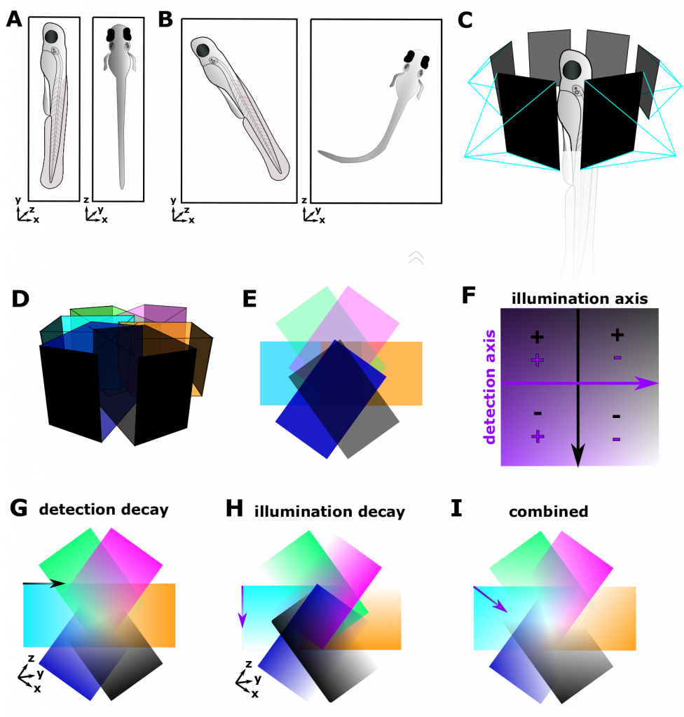
Figure 2: Sample Geometry and Light Paths in a single-sided illumination LSFM. (A) Optimized sample alignment, with respect to sample geometry, reduces image/stack size and decreases the beam path, thus interaction of light with matter. (B) Non-optimum sample alignment, increases image/stack size and thus increases the beam path. (C) Multi-view acquisition from various angles. (D) Stacks acquired from various angles can be digitally fused subsequently. (E) Top-view of (D), representing stack-overlap with ideal image properties. (F) Image properties vary according to the position relative to the detection and illumination axis, i.e. top left quadrant – good illumination and acquisition, bottom right – poor illumination and acquisition. (G) Image z-axis detection decay. (H) Image x-axis illumination decay. (I) Combined detection and illumination decay.
Aligning sample, limiting stack size, and acquisition intervals
When thinking about sample alignment, one also has to consider:
- how much space there is in the sample chamber for the sample (i.e. does the sample fit and how much room for movement do you have),
- how the angle of sample embedding impacts positioning or acquisition (i.e. embedding your sample at an angle might significantly increase stack size, often unnecessarily), and consistency between samples.
- how the acquisition angles themselves impact imaging (i.e. can you capture all the information you need, is there enough information to merge images from multiple views sufficiently, does multiview acquisition really add to your data (see following post)).
When defining your stack size and intervals, consider 4 dimensions:
- XY – Considering voxel and image size is crucial to keep an eye on data size. Especially with small samples or sparse data (e.g. the vasculature), reducing image size can make a huge difference for subsequent data handling. Equally, considering the shape of your sample (e.g. long and thin vs. cubic) influences the shape of your xy-dimensions.
- Z – Even though it can be tempting to have a large step size to reduce imaging time, data in the z-dimension have generally a lower resolution and are impacted by point-spread function [PSF]. Similarly, voxel anistropy (i.e. a voxel is not a cube but a cuboid) can be challenging for image processing. This can be partially addressed by interpolation to make voxels isotropic, but this highly depends on input image quality. Conversely, using minimal step size might produce superflous data, which do not necessarily add to knowlegde but definetely complicate data handling and processing. Together, before imaging consider an accurate sampling frequency, and how this related to your lightsheet thickness (see following post), for your biological question and computational workflow.
- Time – When setting up time-lapses to examine dynamic phenomena, knowing your biological question is key [eg. if cells divide every 20min, do you need to acquire a 3D stack every minute? Or, if cells bleb every minute, would you produce useful data when acquiring every 10 minutes?]. When setting up long time-lapses, it is also worth considering that your sample might grow, resulting in a change of position as well as optical properties (eg. increasing pigmentation, new limb, etc).
Considering the four dimensions will thus influence the quality of data, acquisition time, and data load. Additionally, it will impact the light dosage experienced by the sample, and if optimized, allow longer survival of living samples.
Checking fluorescence and calibration
To calibrate beam path positions, depending on your microscope setup, either the sample chamber, or only the light sheet itself, will need to be aligned to ensure the LS beam waist being aligned with the detection lens focal plane. This is followed by bringing your sample into focus and deciding the optimum LS thickness. Calibration should be made regularly especially when using a facility/shared system. Better calibration, better data!
When examining your imaging setup (i.e. lasers, filters, gains, etc.) ensure that crosstalk and saturation are avoided. Also, homogenous signal should be available throughout the sample (e.g. antibody penetration is limited, and illumination/detection decay will impact this). Also, imaging systems do age. Thus, imaging samples over months may be affected.
Depending on your imaging setup and sample, stripe-artefacts and shadowing can occur. Although these are generally considered artefacts, and can be addressed by pivoting the light sheet, shadowing provides information on signal distribution and object localization. For example, if pigmentation produces shadowing, how meaningful are the data on objects that are positioned behind these pigments? Artefacts are classified by users who do not like to see them, but they represent a normal physical aspect of their sample…maybe another mounting, or protocol could improve them rather than physically “Photoshop” them.
When setting up time-lapses additional considerations need to be met. For example, can environmental conditions be stably maintained (e.g. temperature, acidity, oxygen) and could potential adverse effects arise (e.g. quenching due to anti-fade chemicals, toxic reactions from fluorophores or dyes)? Similarly, it is advisable to image larger FOVs for time-lapses to avoid losing your region of interest by focal drift and motion artefacts.
Together, it becomes clear that myriads of considerations influence the imaging setup and that even though we would like to think about them as optimized, a perfect image can never be achieved due to the unavoidable interaction of light with matter.
May the LISH be with you,
Elisabeth and Emmanuel
P.S.: If you want to share your views, do not hesitate to get in touch.
Associations / Institutes
(1) Institute of Ophthalmology, Faculty of Brain Sciences, University College London, 11-43 Bath Street, LondonEC1V 9EL. (2) School of Biomolecular and Biomedical Science, University College Dublin, Belfield, Dublin 4. Ireland.
Acknowledgements
Gopi Shah and Montserrat Coll Llado for the free and positive review.
Further Reading:
- Jacques, S. (2013). Optical properties of biological tissues: a review. Physics in Medicine & Biology 58(11).
- North, A. (2006). Seeing is believing? A beginners’ guide to practical pitfalls in image acquisition. J Cell Biol. 172(1): 9–18.
- Icha, J., Weber, M., Waters, J., and Norden, C. (2017), Phototoxicity in live fluorescence microscopy, and how to avoid it. Bioessays 39(8).
- Flood, P.M., Kelly, R., Gutiérrez-Heredia, L. and Reynaud, E.G. (2013). ZEISS Lightsheet Z.1 Sample Preparation. ZEISS.
- Flood, P., Page, H., and Reynaud, E. (2016). Using hydrogels in microscopy: A tutorial, Micron 84:7-16.
- Richardson, D. and Lichtman, J. (2015). Clarifying Tissue Clearing. Cell 162(2): 246–257.
 (No Ratings Yet)
Blog series
Have an idea for a blog series?
Filter by
- NewsApply
- DiscussionsApply
- How toApply
- ToolsApply
- Case studiesApply
- InterviewsApply
- JobsApply
- EducationApply
- Blog seriesApply
- Towards Global Acces..sApply
- Latin America Bioima..gingApply
- From Zero to Qupath ..HeroApply
- Asian Microscopists ..and Cell BiologistsApply
- AIC at HHMI JaneliaApply
- Deep Learning for Bi..o-image analysisApply
- GloBIAS – updates fr..om the communityApply
- WAMBIAN: West Africa.. in FocusApply
- Volume EMApply
- Latin American Micro..scopistsApply
- Bio-image Analysis w..ith NapariApply
- Imaging with…Apply
- Highlights from Euro..-BioImagingApply
- LSFM seriesApply
- DIY MicroscopyApply
- View all