Quality assurance of segmentation results

This blog post revolves around determining and improving the quality of segmentation results. A common problem is that this step is often omitted and done rather by the appearance of the image segmentation than by actually quantifying it. This blogpost aims to show different ways to achieve this quantification as this leads to reproducibility.

Therefore, we will see what a segmentation is and where the difference between an instance and a semantic segmentation lies. Furthermore, we will investigate two ways of nuclei segmentation in 3D, namely Voronoi-Otsu-Labeling and StarDist. Later, we will use the-segmentation-game to compare them to a ground truth annotation generated in a previous blogpost.

Segmentation – Instance vs. Semantic

In an image analysis workflow, after preprocessing typically follows the image segmentation.

During segmentation the image is divided into different regions: the background and foreground. Hereby, thresholding is an effective way to separate these groups. Everything below a certain threshold is then considered background (pixel values = 0 or False) and everything above this region is considered foreground (pixel values = 1 or True).

This scenario provides an example of what semantic segmentation is: all objects of the same class are labeled similarly.

Additionally, this foreground class can be subdivided into regions of interest that are labeled with different numbers to differentiate objects within the same class. This is an example of instance segmentation: each object is labeled uniquely.

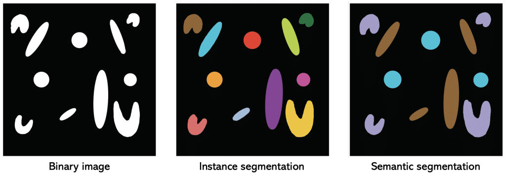
The resulting labeled image (or just ‘label image’) builds the foundation for quantitative analysis.

Note: In the Bio-image Analysis Notebooks, there is a chapter on algorithm-validation.

Requirements

In this blogpost the following napari-plugins are used/mentioned

• napari-pyclesperanto-assistant
• napari-stardist
• the-segmentation-game
• napari-workflow-optimizer

Ground truth annotation

After we looked at how to annotate images in 3D, we want to use these ground truth annotations as a comparison to draw conclusions on the quality of an algorithm’s segmentation result.

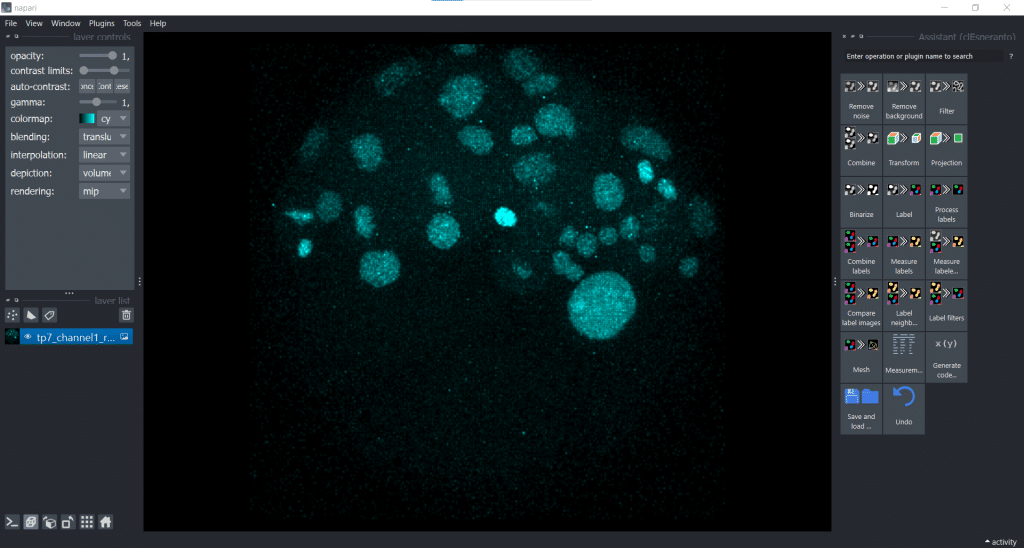
For this, we will explore a dataset of the marine annelid Platynereis dumerilii from Ozpolat, B. et al licensed by CC BY 4.0. We will concentrate on a single timepoint and channel for our segmentation.

The generated ground truth looks like this:

x-y-plane	y-z-plane

Voronoi-Otsu-Labeling

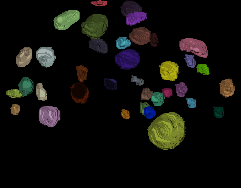
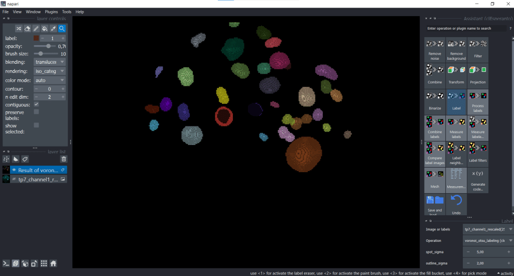
Now, we are generating a segmentation result using Voronoi-Otsu-Labeling. Therefore, we open under Plugins the clesperanto Assistant. The opened assistant should appear at the right side of napari GUI:

Then we can select under Label → Voronoi-Otsu-labeling (nsbatwm). Here we can adjust two sigmas: the spot and the outline sigma. The spot sigma controls the minimal distance between objects and the outline sigma controls the preciseness of the object’s outline. For this example, we select spot_sigma = 5.00 and outline_sigma = 2.00 (see also this related jupyter notebook):

For other planes, the segmentation result looks like this:

x-y-plane	y-z-plane

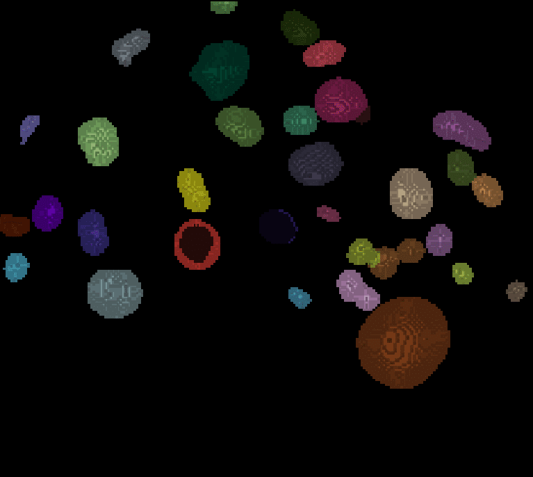StarDist

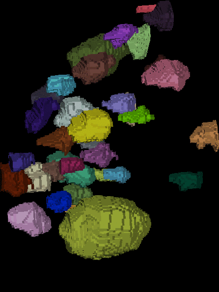
Here, we generate another segmentation result using StarDist. Therefore, we open under Plugins → StarDist (napari-stardist) which looks like this:

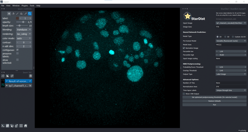
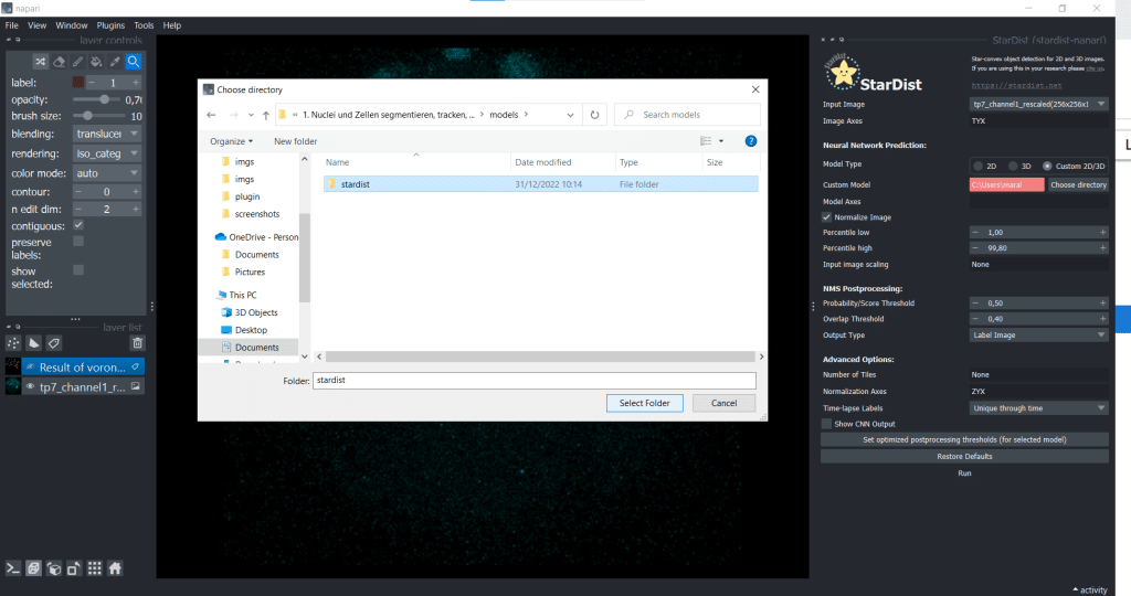
Next, we select the option of importing a self-trained model by selecting Custom 2D/3D. If you are interested in how to train a stardist-model, you can check out the StarDist documentation which hosts jupyter notebooks explaining data requirements, training and prediction in 2D and 3D. Furthermore, this video explains nicely how StarDist works and I added some more information in this notebook which, in my opinion, is helpful. To use Custom 2D/3D in napari, we need to provide a path to a StarDist model folder, as shown below:

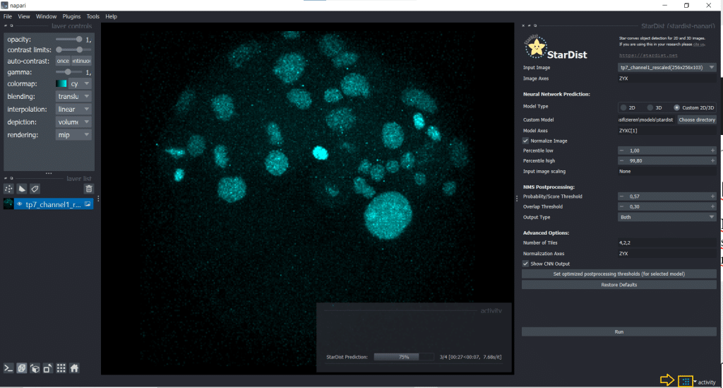
Then, click the button Set optimized postprocessing thresholds (for selected models) and the information about the thresholds will be derived from the tresholds.json file which is also part of the model folder. When you press the Run button, a prediction will be generated fro the model. This can take some time and you can see it on the blue running sign in the bottom right corner:

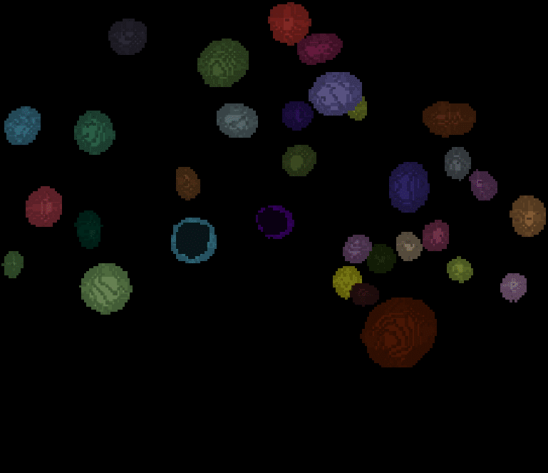
The outputs are four layers containing distances, probabilities, StarDist labels and StarDist polyhedra

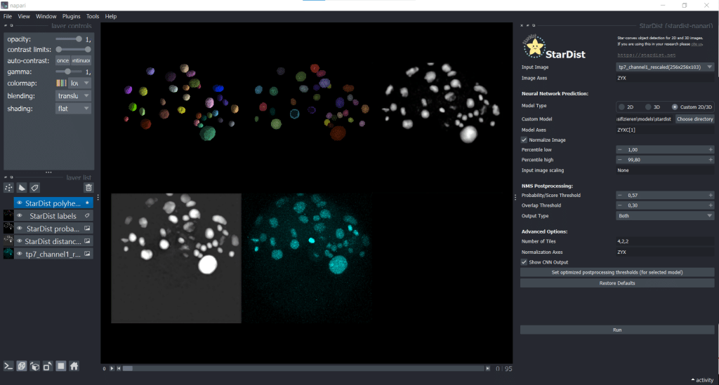
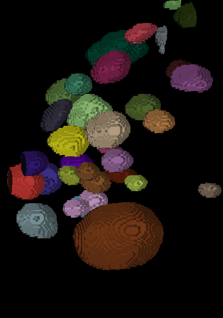
The segmentation result looks like this:

x-y-plane	y-z-plane

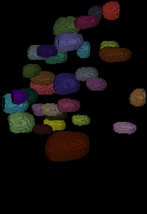Playing the-segmentation-game

Now, we are playing the-segmentation-game. This is a napari-plugin which can be used for parameter tuning of a segmentation algorithm or a segmentation algorithm comparison (see also the-segmentation-game in praxis). Therefore, we go to Tools → Games and select The Segmentation Game.

Parameter tuning

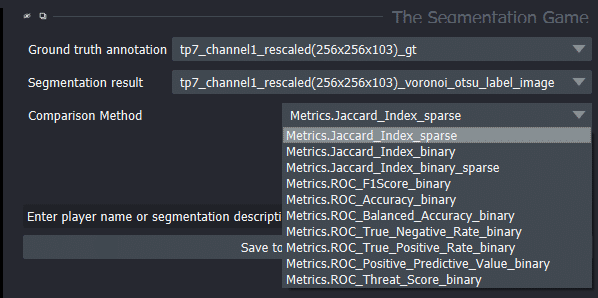
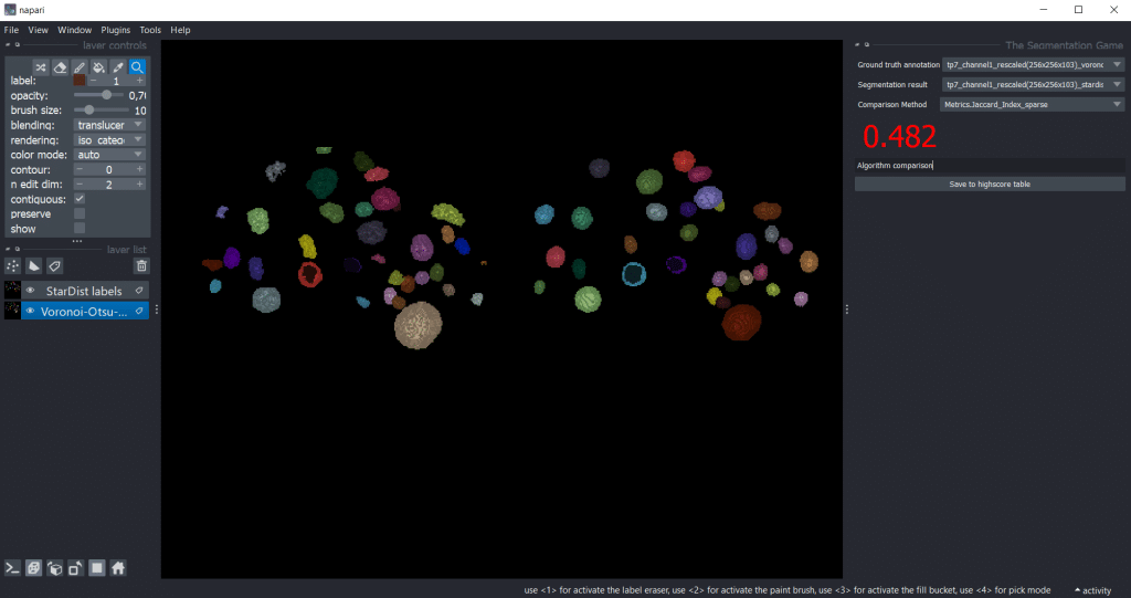
Next, we want to load our ground truth annotation into napari and generate a Voronoi-Otsu-Labeling result as shown above. The-segmentation-game allows us to compare these two using different metrics. One of these implemented metrics is the sparse Jaccard index.

The Jaccard index

The Jaccard Index is a measure to investigate the similarity or difference of sample
sets. Hereby, the so called sparse Jaccard Index measures the overlap lying between
0 (no overlap) and 1 (perfect overlap). Therefore, the ground truth label is compared
to the segmented label by determination of the maximum overlap. The metric result is
the mean overlap of all investigated labels (Jaccard, 1902) (see this jupyter notebook).

Beside the sparse Jaccard index, there is also the binary Jaccard index. If you are interested in the difference, see this jupyter notebook.

With the help of the sparse Jaccard index, we can fine-tune our Voronoi-Otsu-Labeling result by adjusting the spot_sigma and the outline_sigma:

We can also choose other quality metrics in the-segmentation-game:

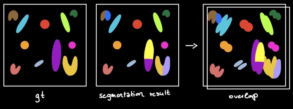
Demonstration of quality metrics

In the following video we use a minimal example to understand these different metrics (sound on 😊 ):

Another way to look at true positives (TP), true negatives (TN), false positives (FP) and false negatives (FN) is to visualize them in a confusion matrix.

Confusion matrix

Another way to look at true positives (TP), true negatives (TN), false positives (FP) and false negatives (FN) is to visualize them in a confusion matrix.

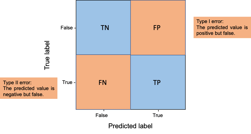
In the context of segmentation, this means:

• TP are pixels which are in ground truth (gt) foreground (1) and in the segmentation result foreground (1)
• TN are pixels which are in gt background (0) and in the segmentation result background (0)
• FP are pixels which are in gt background (0) but in the segmentation result foreground (1)
• FN are pixels which are in gt foreground (1) but in the segmentation result background (0)

Out of these values, accuracy, precision and recall can be computed as shown already in the video above. If you are more the reading than listening person, you can check out what they mean in the following sections.

Accuracy

On the one hand, the accuracy score displays the ratio of the sum of TP and TN out of all predictions. It is a measurement that closely agrees with the accepted value. We basically ask: How well did my segmentation go regarding my two different classes (foreground and background)?

Accuracy = (TP + TN)/(TP + FN + TN + FP)

Precision

On the other hand, the precision score is the count of TP out of all positive predictions. It agrees with other measurements in the sense that they show similarities with each other. We basically ask: How well did my segmentation go regarding the prediction of foreground objects?

Precision = (TP)/(TP + FP)

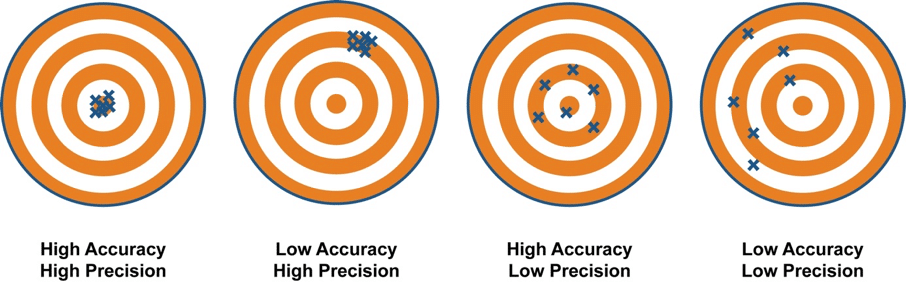
The difference between accuracy and precision is visualized here:

Recall

The Recall score  is the true positive rate (TPR) aka Sensitivity. It is measuring the count of TP out of all actual positive values. We basically ask: How many instances were correctly identified as foreground?

Recall = (TP)/(TP+FN)

F1-Score

The F1-score is the harmonic mean between precision and recall score. It can be used as a compromise when choosing between precision and recall score. This results in a trade-off between high false-positives and false-negative rates (see also this book).

F1-Score = 2 x ((precision x recall) / (precision + recall))

For more information on the shown metrics and a little exercise, check out this jupyter notebook.

Segmentation algorithm comparison

We can also use the-segmentation-game to compare segmentation results. Therefore, we need to select one segmentation result as Ground truth annotation and the other one as Segmentation result.

Generally, we can get the output for all quality metrics using the highscore table by pressing Save to highscore table. For the example shown in the blogpost, we got the following highscore tables:

description	GT vs. Voronoi-Otsu-Labeling result	GT vs StarDist labels	Voronoi-Otsu-Labeling result vs. StarDist labels
ground_truth_annotation	gt	gt	voronoi_otsu_label_image
segmentation_result	voronoi_otsu_label_image	stardist_label_image	stardist_label_image
Jaccard_Index_sparse	0.584	0.490	0.482
Jaccard_Index_binary	0.708	0.551	0.549
Jaccard_Index_binary_sparse	0.000	0.012	0.000
F1Score_binary	0.829	0.711	0.709
Accuracy_binary	0.995	0.991	0.991
Balanced_Accuracy_binary	0.894	0.846	0.862
True_Negative_Rate_binary	0.998	0.996	0.995
True_Positive_Rate_binary	0.791	0.696	0.730
Positive_Predictive_Value_binary	0.871	0.725	0.700
Threat_Score_binary	0.710	0.551	0.549

Conclusion

When we reflect on the example which is shown throughout the blog post, we see that our Voronoi-Otsu-Labeling result and our StarDist result are differing which might be related to the way I annotated the ground truth for the StarDist model. For further workflow steps, it would make sense to set a threshold and use a segmentation result with e.g. Jaccard index (sparse) ≥ 0.7. For this example, neither the Voronoi-Otsu-Labels nor the StarDist labels fulfill this condition. We would need to use another segmentation algorithm or retrain the StarDist model.

But from just looking at the segmentation result, we probably don’t know that the segmentation result is insufficient. And even if we know, it makes more sense to quantify the quality of the segmentation to be sure it can be used further, for example for deriving measurements and plotting.

Further ideas

Here are some other ideas how we can determine the quality of our segmentation:

• Use object (e.g. nuclei) count manually and automatically. → Use accuracy, precision, recall and/or F1-score (also here the scores need to be over a certain threshold to be used in later image-analysis-steps).

• Calculate the centroid distance between two overlapping images. → The higher the distance the worse is the segmentation result.

• Metrics Reloaded addresses the problem of choosing the right performance metrics in very detail. They also developed an online tool which helps choosing a proper validation metric and allows exploring strengths and weaknesses of common metrics.

• Another plugin which I briefly want to mention if you aim to optimize your image processing workflow for segmentation quality is the napari-workflow-optimizer. If you want to see an application example, have a look into this jupyter notebook.

Further reading

• Metrics reloaded: Pitfalls and recommendations for image analysis validation. Maier-Hein L. and Reinke A. et al.
• Sklearn: Metrics and scoring
• Metrics to investigate segmentation quality

Feedback welcome

Some of the napari-plugins used above aim to make intuitive tools available that implement methods, which are commonly used by bioinformaticians and Python developers. Moreover, the idea is to make those accessible to people who are no hardcore-coders, but want to dive deeper into Bio-image Analysis. Therefore, feedback from the community is important for the development and improvement of these tools. Hence, if there are questions or feature requests using the above explained tools, please comment below, in the related github-repo or open a thread on image.sc. Thank you!

Acknowledgements

I want to thank Dr. Robert Haase, Prof. Martin Schätz, Dr. Uwe Schmidt and Dr. Martin Weigert as the developers behind the tools shown in this blogpost. This project has been made possible by grant number 2022-252520 from the Chan Zuckerberg Initiative  DAF, an advised fund of the Silicon Valley Community Foundation. This project was supported by the Deutsche Forschungsgemeinschaft under Germany’s Excellence Strategy – EXC2068 – Cluster of Excellence “Physics of Life” of TU Dresden. 

Reusing this material

This blog post is open-access, figures and text can be rused under the terms of the CC BY 4.0 license unless mentioned otherwise.

(5 votes, average: 1.00 out of 1)