Feature extraction in napari
Posted by Mara Lampert, on 3 May 2023
This blog post revolves around extracting and selecting features from segmented images. We will define the terms feature extraction and selection. Also, we will learn how to categorize features and can look up specific features in a glossary. Furthermore, we will explore how to extract features in napari.
Definition of feature extraction
During feature extraction, quantitative measurements are assigned to image sets, images or image regions. Feature type involves both feature detection and feature
description. Importantly, features should be independent
of location, rotation, spatial scale or illumination levels (Gonzalez and Woods, 2018).
Nevertheless, there are connections, e.g between location and position, spatial scale and size as well as illumination levels and intensity that one needs to be aware of.
Categories of features
We can differentiate features into different categories:
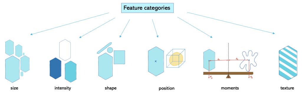
Size (siz)-based parameters relate to magnitude or number of dimensions. Examples are area and volume.
Intensity (int)-based parameters are all parameters related to the power transferred per unit area. Examples are minimum, mean, maximum intensity.
Shape (sh) -based parameters refer to the geometry of the object and relate to the outline of the object and surface. Examples are roundness, aspect ratio and solidity.
Position (po)-based parameters refer to where an object is at a particular time. This is specified relative to a frame of reference.
Moment (mom)-based parameters refer to a physical quantity which has a certain distance from a reference point. Hereby, the moment relates to the location or arrangement of the physical quantity. Typically, these physical quantities are forces, masses or electric charge distributions. One example is torque which is the moment of force.
Texture (tex)-based parameters relate to the crystallographic orientation within a sample. It can be described as random, weak, moderate or strong texture depending on the amount of objects with the preferred orientation. An example is standard deviation of intensity.
Note: In the Bio-image Analysis Notebooks, there is a chapter on feature extraction.
Glossary
This is a collection of features provided by napari-skimage-regionprops (nsr) and napari-simpleitk-image-processing (n-SimpleITK). Hereby, note that some of the mentioned parameters may be implemented differently in both libraries.
| feature | schematics | category | explanation | formula | implementation |
| area (or volume in 3D) |   | siz | = sum of pixels/ voxels of the region scaled by pixel-area/ voxel-volume. | 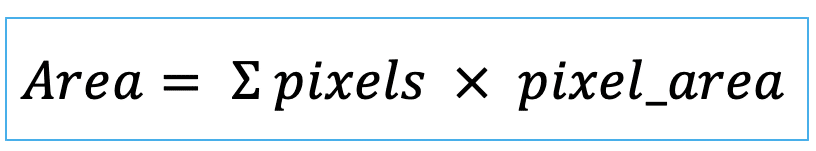  | nsr |
| aspect_ratio | 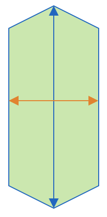 | sh | = the ratio between object width and object length. |  | nsr |
| bbox | 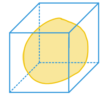 | po | = minimum range in each spatial dimension | 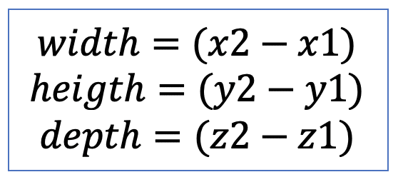 | nsr |
| bbox_area (or bbox_volume in 3D) | 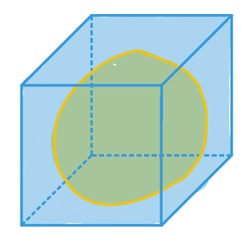 | siz | = number of pixels/ voxels of bounding box scaled by pixel-area/ voxel-volume | 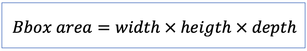 | nsr |
| centroid | 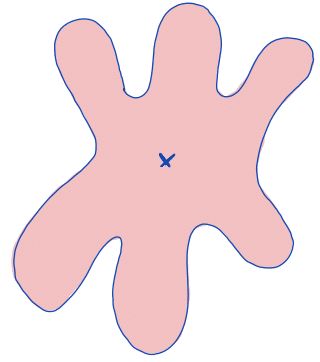 | po | = geometric center. It is the arithmetic mean position of all points in the surface of the figure. Therefore, the x and y coordinates of all image pixels are averaged. | 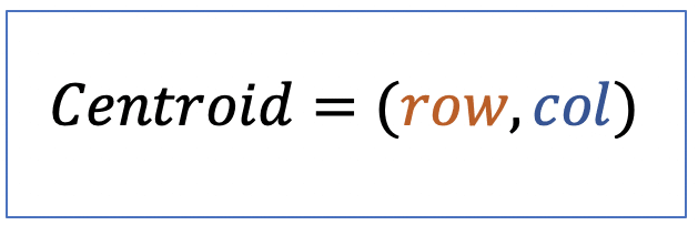 | nsr |
| circularity | 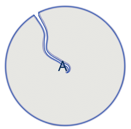 | sh | =the area-to-perimeter-ratio. It takes local irregularities into account. | 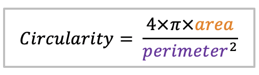 | nsr |
| convex_area | 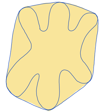 | siz | = area of the convex hull of the region. (only available in 2D) | nsr | |
| convex hull | 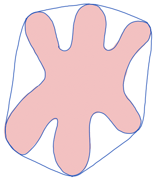 | siz | = smallest region that is convex and contains the original region. | ||
| eccentricity | 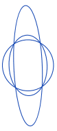 | sh | = describes how “elongated” a shape is compared to a perfect circle. | 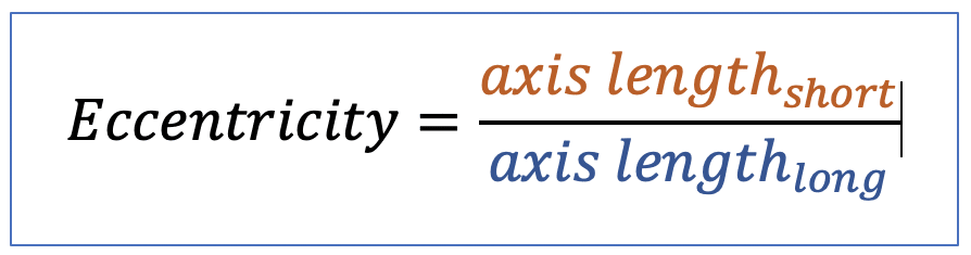 | nsr |
| elongation |  | sh | = ratio between length and width of the object bounding box | 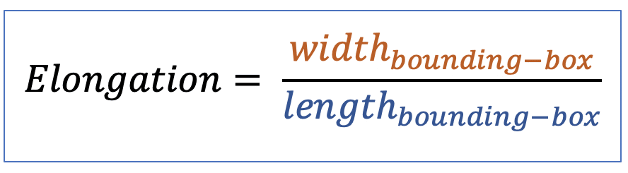 | n-SimpleITK |
| equivalent_diameter | 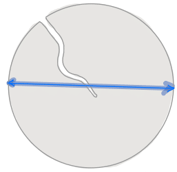 | siz | = diameter of a circle with same area as region. | nsr | |
| equivalent_ellipsoid_diameter | 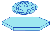 | siz | = diameter of an ellipsoid that has the same volume as the object. | uses principal axes for computation | n-SimpleITK |
| equivalent_spherical_perimeter | 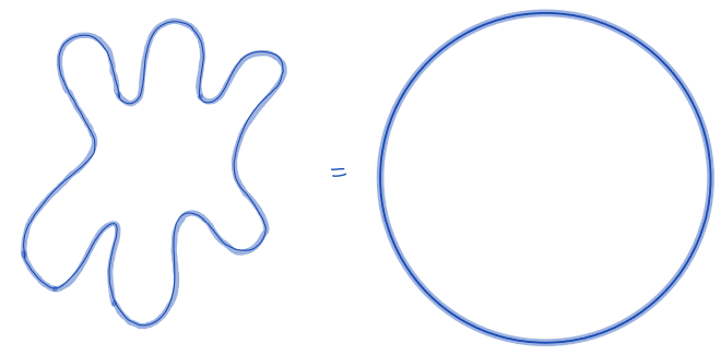 | siz | = comparison of the perimeter of the object with the perimeter of a sphere with similar geometric properties. | n-SimpleITK | |
| equivalent_spherical_radius | 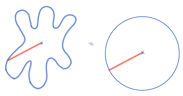 | siz | = comparison of the radius of the object with the equivalent radius of a sphere with similar geometric properties | n-SimpleITK | |
| extent | 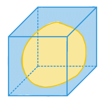 | po/ siz | = Ratio of pixels in region to pixels in the total bounding box. | 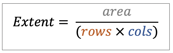 | nsr |
| feret_diameter | 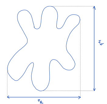 | sh | = distance between the two parallel planes restricting the object perpendicular to that direction | n-SimpleITK | |
| feret_diameter_max | 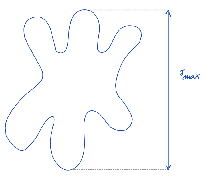 | sh | = longest distance between points around a region’s convex hull contour (only available in 2D) | nsr | |
| flatness | 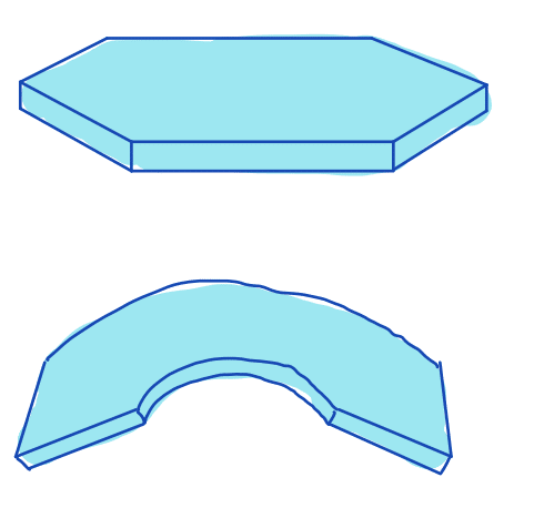 | sh | = degree to which the surface of the object approximates a mathematical plane | n-SimpleITK | |
| local_centroid | po | = average location of all the points within bbox of the region. | 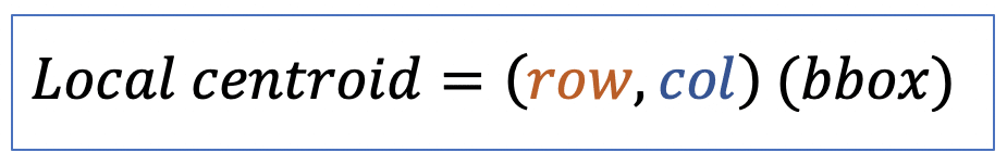 | nsr | |
| major_axis_length |  | sh | = longest diameter. It is a line segment that passesthrough the center as well as both foci and terminates at the two points on the perimeter that are the furthest apart. Therefore, it is a measure of object length. | nsr | |
| max_intensity/ maximum |  | int | = highest intensity value in the region | nsr/ n-SimpleITK | |
| mean_intensity/ mean |  | int | = mean intensity value in the region | nsr/ n-SimpleITK | |
| median | int | = median intensity value in the region | n-SimpleITK | ||
| min_intensity/ minimum |  | int | = lowest intensity value in the region | nsr/ n-SimpleITK | |
| minor_axis_length |  | sh | = shortest diameter. It is a line segment that passes through the center and terminates at the two points on the perimeter that are closest to one another. Therefore, it is a measure of object width. | nsr | |
| moments | mom | = Spatial moments up to 3rd order | m_ij = sum{ array(row, col) * row^i * col^j } | nsr | |
| moments_central | mom | = Central moments (translation invariant) up to 3rd order. | mu_ij = sum{ array(row, col) * (row - row_c)^i * (col - col_c)^j } | nsr | |
| moments_hu | mom | = Hu moments (translation, scale and rotation invariant) | nsr | ||
| moments_normalized | mom | = Normalized moments (translation and scale invariant) up to 3rd order | nu_ij = mu_ij / m_00^[(i+j)/2 + 1] | nsr | |
| number_of_pixels (or number of voxels in 3D) | siz | = count of pixels/ voxels within a label |   | n-SimpleITK | |
| number_of_pixels_on_border (or number of voxels on border in 3D | siz | = count of pixels/ voxels within a label that is located at the image border | n-SimpleITK | ||
| orientation | 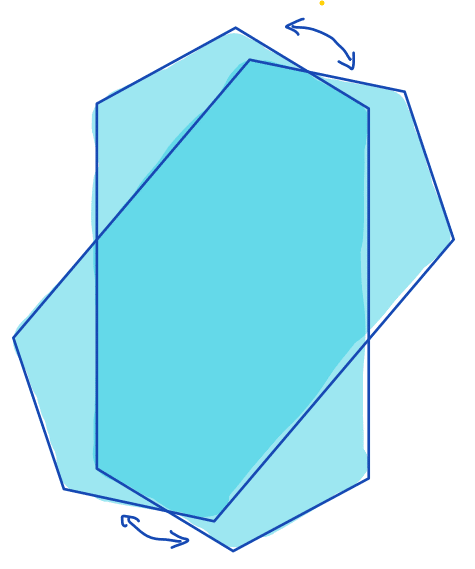 | po | = overall direction of shape. It is calculated as the angle between the major axis of an ellipse that has same second moments as the region and a reference axis, such as the x-axis. | nsr | |
| perimeter |  | siz/ sh | = uses a 4- connectivity to represent the contour as a line through the center of border pixels (only available in 2D) | nsr/ n-SimpleITK | |
| perimeter_crofton | sh | = perimeter approximated by Crofton formula in 4 directions (only available in 2D) | nsr | ||
| perimeter_on_border | sh | = number of pixels in the objects which are on the border of the image (only available in 2D) | n-SimpleITK | ||
| perimeter_on_border_ratio | sh | = describes the ratio between the number of pixels at the image border divided by the number of pixels on the object’s perimeter (only available in 2D) | n-SimpleITK | ||
| principal_axes | mom | = Principal (major and minor) axes are those axes passing through the centroid, about which the moment of inertia of the maximal or minimal region. It is the axis around which the object rotates the easiest or the most stable. | n-SimpleITK | ||
| principal_moments | mom | = values that describe how much the object resists rotation around each of its principal axes. | n-SimpleITK | ||
| roundness | 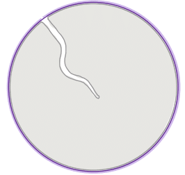 | sh | = describes the area-to-perimeter- ratio. In contrast to circularity it excludes local irregularities by using the convex perimeter instead of the perimeter. | 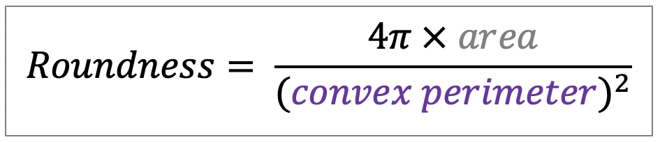 | nsr/n-SimpleITK |
| sigma (intensity) | int | = information on structure scale or local contrast (higher values → smoother/ more globally homogeneous region; lower values → sharper/ more locally distinct structures. | n-SimpleITK | ||
| solidity | 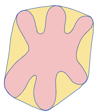 | sh | = measures the density of an object. (only available in 2D) | 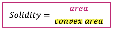 | nsr |
| standard_deviation_intensity | tex | = standard deviation of gray values used to generate the mean gray value. | nsr | ||
| sum (intensity) | int | = sum of the intensity values in the region | n-SimpleITK | ||
| variance (intensity) | int | = measure of dispersion of numbers from their average value | n-SimpleITK | ||
| weighted_centroid | po | = some parts of an object get higher ‘weight’ than others. Therefore, the centroid coordinate is weighted with the intensity image. | nsr |
Feature extraction in napari
Now, we use napari to extract features using an image and a label image.
Requirements
Note: I would recommend to install devbio-napari. It is a collection of Python libraries and Napari plugins maintained by the BiAPoL team, that are useful for processing fluorescent microscopy image data. Importantly, it contains napari-plugins we use in this blog post. If you need help with the installation, check out this blogpost.
In the following paragraphs, we are going to use the following napari-plugins:
- napari-skimage-regionprops (nsr)
- napari-simpleitk-image-processing (n-SimpleITK)
- morphometrics
- napari-accelerated-pixel-and-object-classification (APOC)
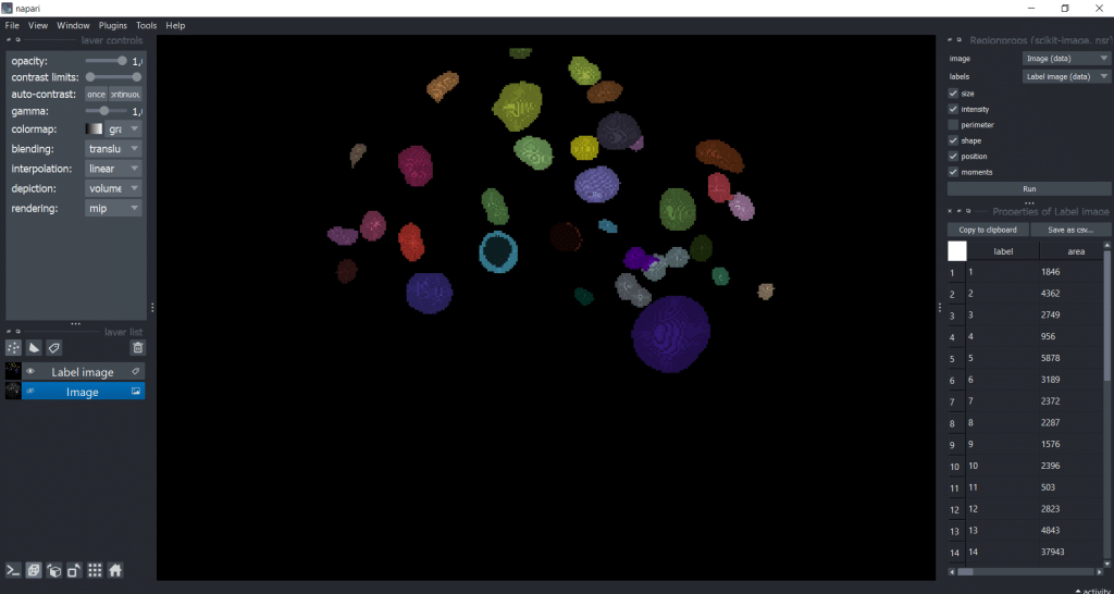
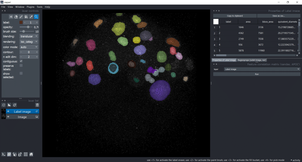
Now, we will explore a dataset of the marine annelid Platynereis dumerilii from Ozpolat, B. et al licensed by CC BY 4.0. When we open our image and our label image in napari in the gallery view, it looks like this:
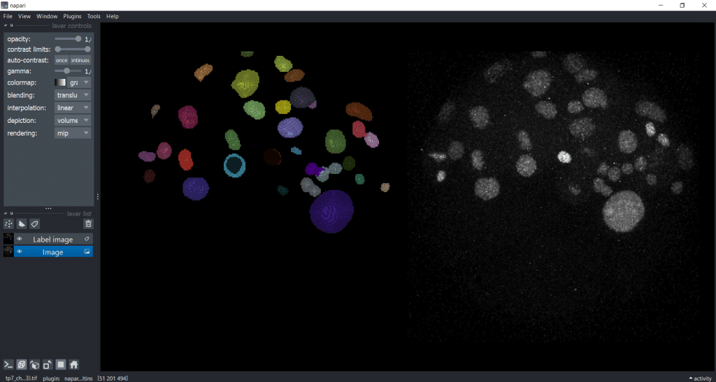
As you can see, the image is 3D and we are concentrating on a rescaled single timepoint and channel for our feature extraction.
Napari-skimage-regionprops
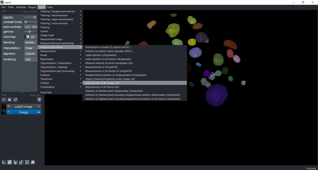
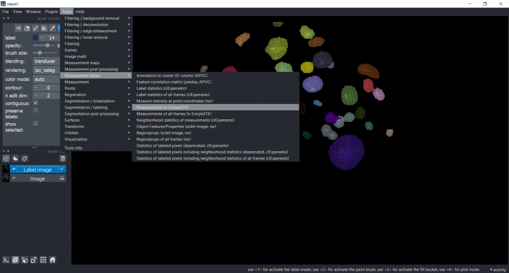
First, we select Tools → Measurement tables → Regionprops (nsr):
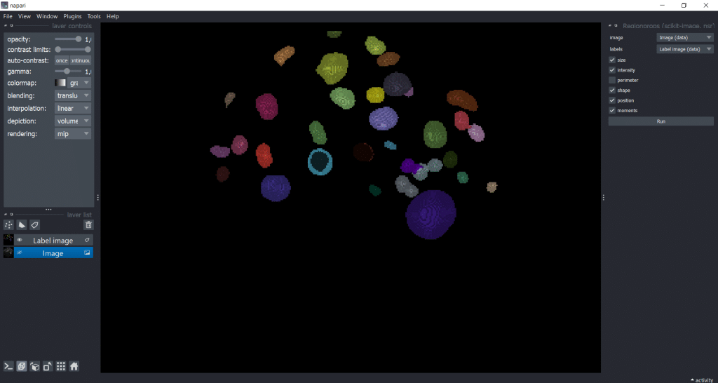
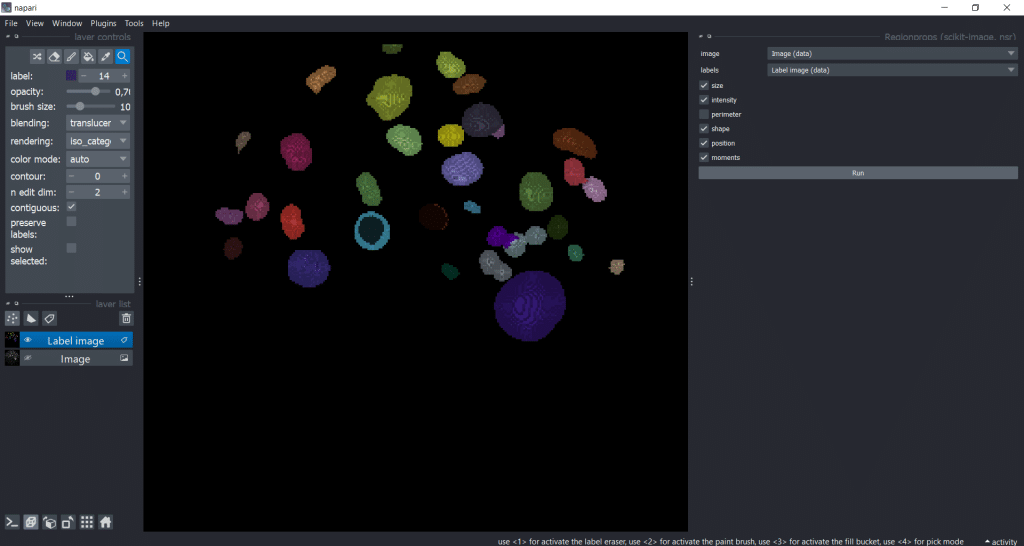
Next, we can select the image, the labels as well as the feature categories that we want to measure. Note that perimeter
-based parameters are not supported in 3D, so we cannot measure them in this example dataset:
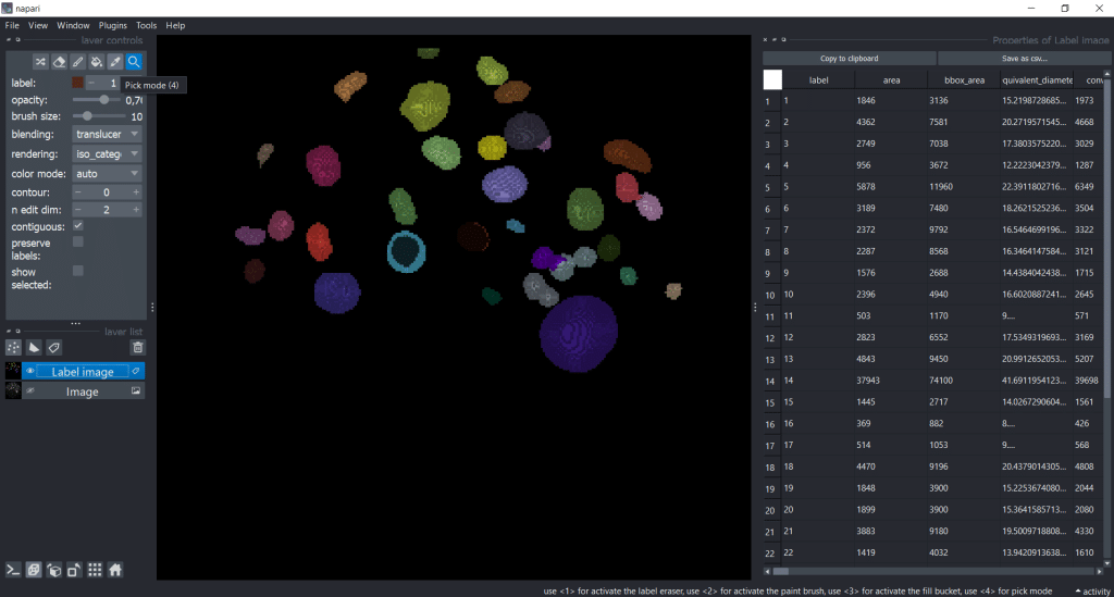
Our output is a table with all parameters:
We can save the table by clicking Save as csv.... Let us close the Regionprops (scikit-image, nsr) window by clicking on the eye symbol. That way we have more space for the table. Personally, I like to increase the table window to have a better overview:
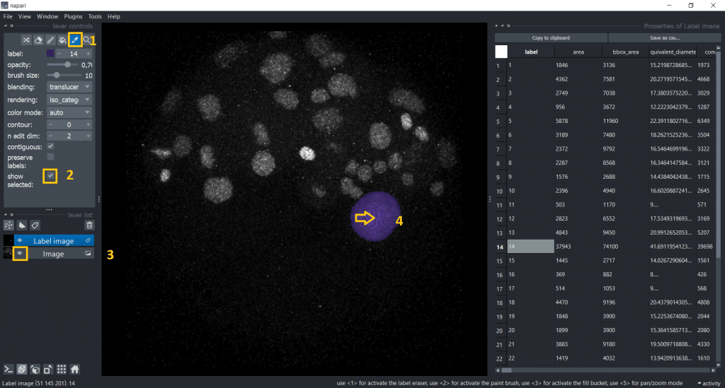
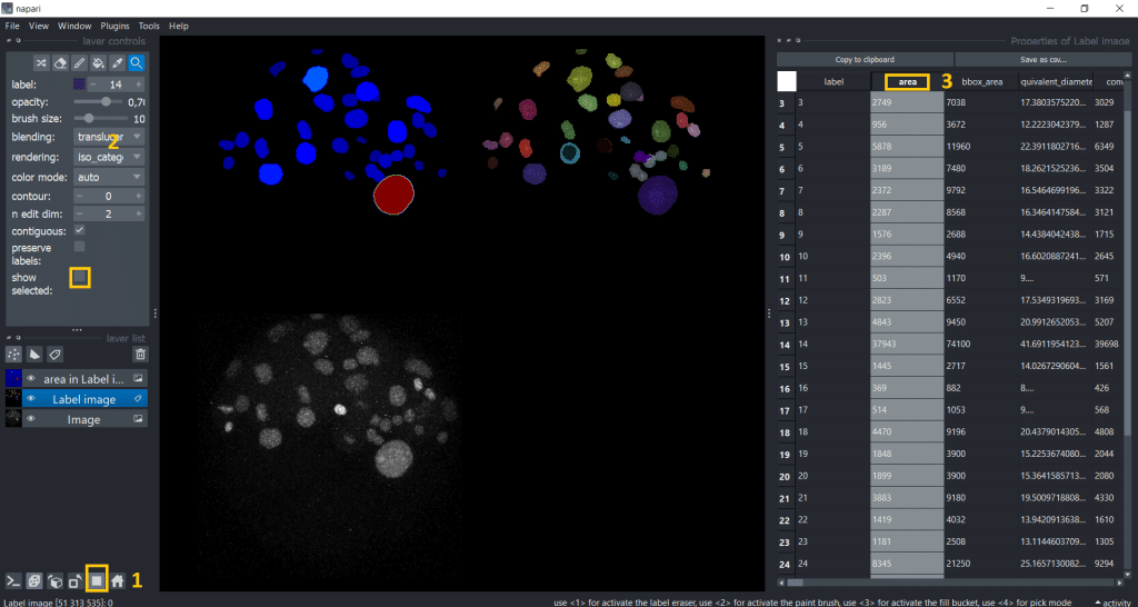
Next, we are interested in individual labels. To visualize them individually, we can
- Activate the
Pick mode (4) - Make the image visible again
- Tick the
show selectedcheckbox - Click on an object we are interested in
Now, we see only the label we selected and the row in the table it corresponds to:
The cool thing is that if we click on another label, it will be automatically updated in the image and table:
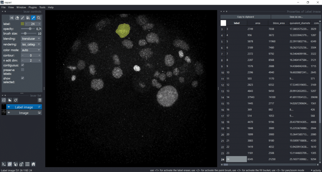
Interestingly, the first object we clicked on seems to be way bigger than the rest. Lets visualize the area of all labels to investigate this. Therefore, we can double click the table header and get a visualization.
For better understanding and visibility, let us:
- Go into gallery view
- Untick the
show selectedcheckbox. In this way, we can see again all labels in the label image - Double click on the table header of the column we want to investigate
The default colormap is called jet which I personally find sometimes confusing, so I will change the colormap to plasma. But you have plenty of colormaps to choose from under layer controls → colormap:
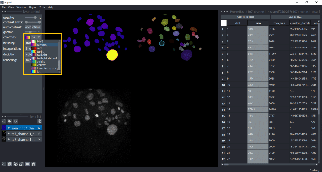
Personally, choosing a colormap that is easy to understand helps me to explore features more easily.
Analyzing timelapse data with napari-skimage-regionprops
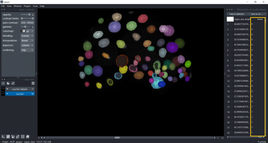
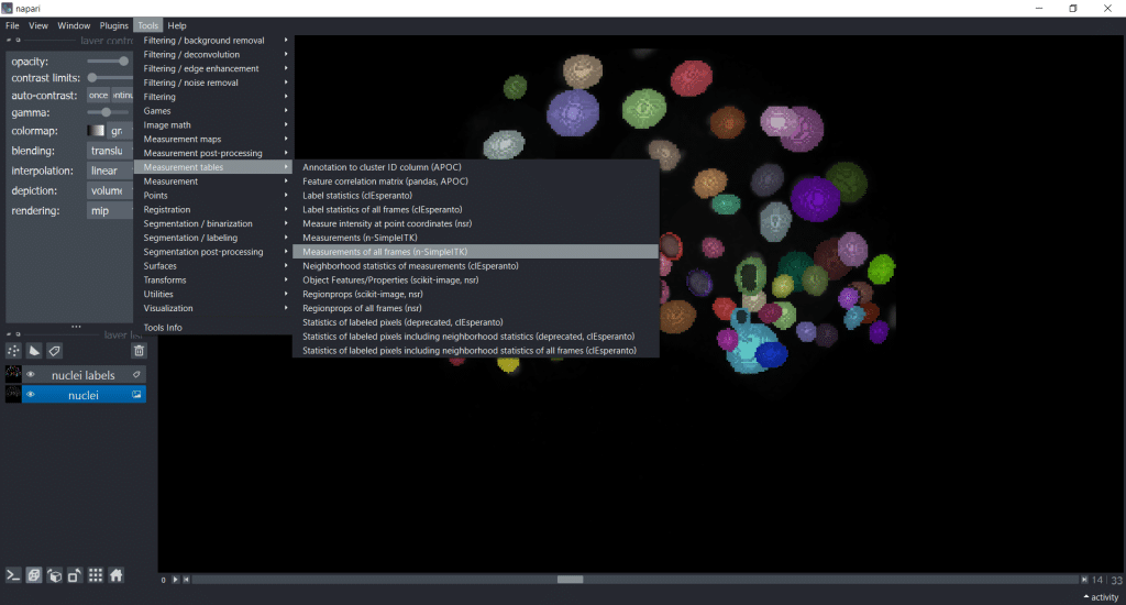
If we are analyzing a timelapse dataset with several frames, we need to select Tools → Measurement tables → Regionprops of all frames (nsr):
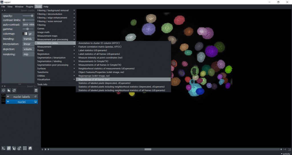
Now, you have a table with a column named “frame”. Hereby, note that if you want to import a custom table into napari, you also need to provide this “frame” column to specify the timepoint:
Note: For more in-depth information, see also the documentation of napari-skimage regionprops.
Napari-simpleitk-image-processing
You can get the measurement table under Tools → Measurement tables → Measurements (n-SimpleITK) :
Again, perimeter-based parameters are not supported in 3D. So, for this example we are measuring all other feature categories.
The following steps are exactly the same as for napari-skimage-regionprops (see above)
Analyzing timelapse data with napari-simpleitk-image-processing
If you are working with timelapse data, then select Tools → Measurement tables → Measurements of all frames (n-SimpleITK) :
Note: This plugin also provides filters and segmentation algorithms. You can find them under
Tools. They have the suffix(n-SimpleITK). See the documentation of napari-simpleitk-image-processing for more detailed information
Morphometrics
You can install morphometrics for example via mamba:
Installation instruction:
mamba install morphometrics -c conda-forge
Morphometrics allows us to get the parameters from these two plugins and the plugin napari-pyclesperanto-assistant at the same time. You can find this option under Tools → Measurement tables → Region properties (morphometrics):
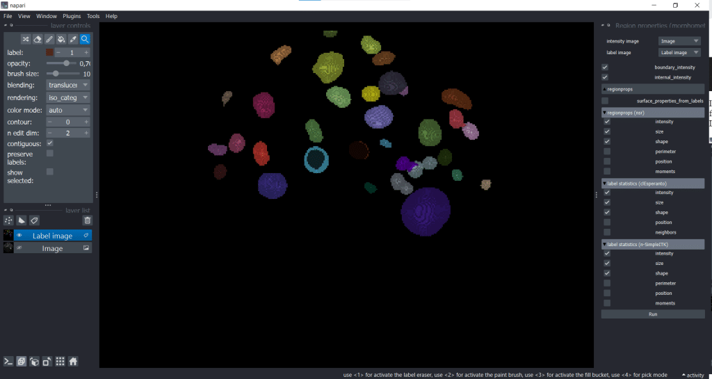
After you selected all measurements you want to derive, just hit the Run button and you will get a table with all measurements like in the examples above.
Using correlation matrices to reduce the number of features
If we now have a table with lots of parameters, it might make sense to investigate whether they are similar to reduce the number of features. We can investigate the similarity of features using correlation filtering. Hereby, our aim is to reduce the number of dimensions for consideration in a given dataset which is called dimensionality reduction.
In napari, we can use napari-accelerated-pixel-and-object-classification (APOC) to get a Feature correlation matrix. We can find it under Tools → Measurement tables → Feature correlation matrix (pandas, APOC). Then, we need to select our Label image as layer:
After pressing the run button, we receive a correlation matrix:
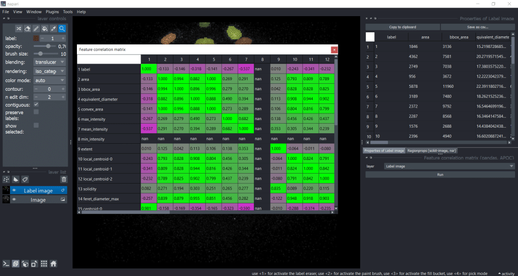
Now, we can investigate which features are strongly correlating. By setting a threshold (e.g. to 0.95), we could select one of these strongly correlating measurements for downstream analysis. For example area and bbox_area are correlation with a factor of 0.994, so it would make sense to only choose one of them .
If you are later on interested to plot your measurements in napari, you can read the FocalPlane post “Explorative image data science with napari” by Robert.
Handling csv-files in napari
If you want to open a csv-file in napari, use Tools → Measurements → Load from csv (nsr).
Furthermore, you can reopen closed tables with Tools → Measurements → Show table (nsr).
A few things I would like to share with you along the way
- Know the features you are working with.
- Features can be implemented differently depending on the library.
- When you don’t understand what a feature means, the best way to figure out is writing a jupyter notebook to test and visualize it.
- It is important to know which range your feature can have, so you avoid measuring nonsense.
Further reading
- Gonzalez, R.C., Woods, R.E., 2018. Digital image processing, Fourth edition, global
edition. ed. Pearson, New York, NY. - Hall, M.A. (2000). Correlation-based feature selection of discrete and numeric class
machine learning. (Working paper 00/08). Hamilton, New Zealand: University of
Waikato, Department of Computer Science. - Imagej glossary of some features
- Scikit-image regionprops documentation
- Lecture slides “Shape Analysis & Measurement” by Michael A. Wirth, Ph.D., University of Guelph, Computing and Information Science, Image Processing Group, © 2004
- Lecture slides “Feature Extraction in Python” by Allyson Quinn Ryan, PhD
- FocalPlane post “Explorative image data science with napari” by Dr. Robert Haase
Feedback welcome
Some of the napari-plugins used above aim to make intuitive tools available that implement methods, which are commonly used by bioinformaticians and Python developers. Moreover, the idea is to make those accessible to people who are no hardcore-coders, but want to dive deeper into Bio-image Analysis. Therefore, feedback from the community is important for the development and improvement of these tools. Hence, if there are questions or feature requests using the above explained tools, please comment below, in the related github-repo or open a thread on image.sc. Thank you!
Acknowledgements
I want to thank Dr. Marcelo Zoccoler, Dr. Robert Haase and Dr. Kevin Yamauchi as the developers behind the tools shown in this blogpost. This project has been made possible by grant number 2022-252520 from the Chan Zuckerberg Initiative DAF, an advised fund of the Silicon Valley Community Foundation. This project was supported by the Deutsche Forschungsgemeinschaft under Germany’s Excellence Strategy – EXC2068 – Cluster of Excellence “Physics of Life” of TU Dresden.
Reusing this material
This blog post is open-access, figures and text can be reused under the terms of the CC BY 4.0 license unless mentioned otherwise.
 (3 votes, average: 1.00 out of 1)
Get involved
Create an account or log in to post your story on FocalPlane.
More posts like this


Filter by
- NewsApply
- DiscussionsApply
- How toApply
- ToolsApply
- Case studiesApply
- InterviewsApply
- JobsApply
- EducationApply
- Blog seriesApply
- Towards Global Acces..sApply
- Latin America Bioima..gingApply
- From Zero to Qupath ..HeroApply
- Asian Microscopists ..and Cell BiologistsApply
- AIC at HHMI JaneliaApply
- Deep Learning for Bi..o-image analysisApply
- GloBIAS – updates fr..om the communityApply
- WAMBIAN: West Africa.. in FocusApply
- Volume EMApply
- Latin American Micro..scopistsApply
- Bio-image Analysis w..ith NapariApply
- Imaging with…Apply
- Highlights from Euro..-BioImagingApply
- LSFM seriesApply
- DIY MicroscopyApply
- View all