Tracking in napari

Posted by Mara Lampert, on 1 June 2023

In this blog post we are exploring cell tracking in napari. Two important processes in normal tissue development and disease are cell migration and proliferation. To gain a better understanding on these processes, tracking in time-lapse datasets is needed. By measuring track properties, like velocity and the total travelled distance, spatio-temporal relationships can be studied. This helps to detect cell-lineage changes resulting from cell division or cell death.

Definition of Tracking

Def. Tracking: Tracking is the motion-analysis of individual objects over space and time. Hereby a unique number for each detected object is generated and maintained.

In a biological context, these individual objects can exemplary be particles (single particle tracking) and cells (cell lineages during development).

Matching and linking

Tracking can be done in different ways depending on the field of application. For instance, we can use a segmentation result or coordinates. Therefore, we take a closer look on the difference between overlap- and coordinate-based tracking.

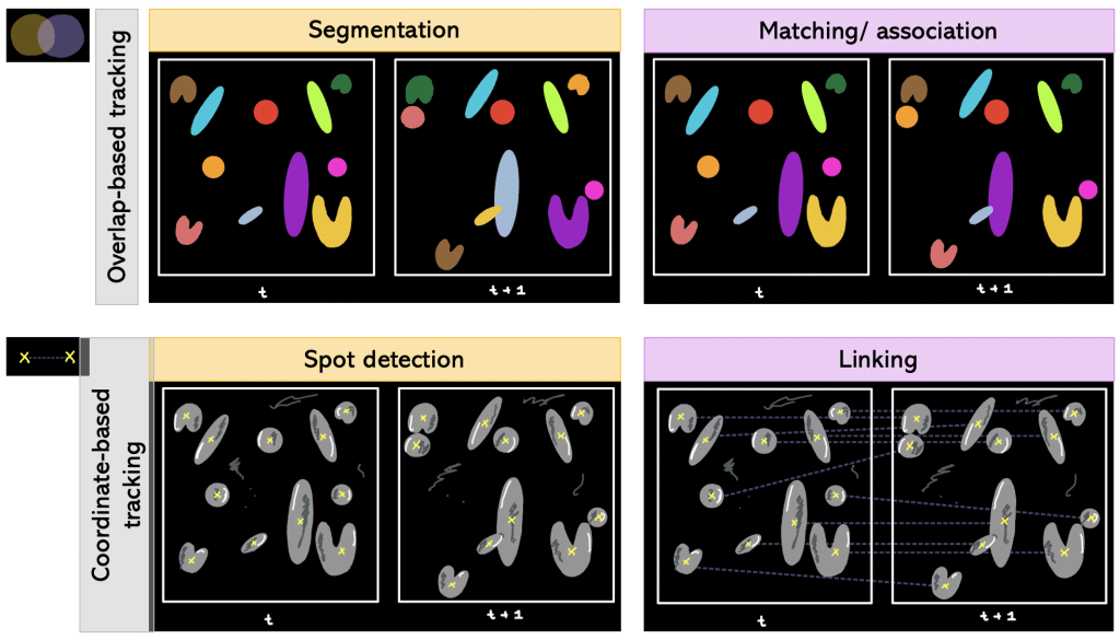
Different ways of tracking: **Segmentation + Matching/association** and **Spot detection + Linking**

Def. Overlap-based tracking: Tracking by overlap between cellular regions in consecutive frames.

Segmentation + matching/association falls under overlap-based tracking.

Def. Segmentation + matching/association: Segmenting every timepoint and matching objects from one timepoint to another. More precisely, it is determined which object in frame number 1 corresponds to which object in frame number 2 (e.g object number 1 in frame 1 corresponds to object number 5 in frame 2).

Besides overlap-based tracking, there is also coordinate-based tracking.

Def. Coordinate-based tracking: Tracking by Euclidean distance between coordinates, e.g. centroids, of detected objects of two consecutive frames in the time-lapse. The generated Euclidean distance is compared to a threshold value: if it is lower than the threshold, it is the same object in motion; otherwise assign new object number.

Spot detection + linking falls under coordinate-based tracking.

Def. Spot detection + linking: Having coordinates in each timepoint and then linking the coordinates of different timepoints together.

Contour evolution and detection methods

We can also differentiate between the different order of steps within the tracking workflow.

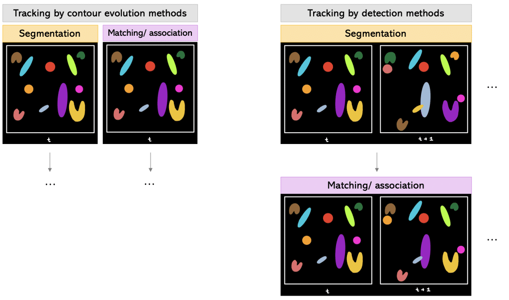
Workflow differences: ***Tracking by contour evolution methods*** and ***Tracking by detection methods***

One way is to track by contour evolution methods.

Tracking by contour evolution methods: Hereby, segmentation and tracking is done frame-by-frame simultaneously. The general assumption is that there is unambiguous, spatiotemporal overlap between the corresponding cell regions.

Another way is to track by detection methods.

Tracking by detection methods: In this approach, first the segmentation is done on all frames. Later, temporal connections between the segmented objects are established using two-frame or multiframe sliding windows.

Next, we want to try out different tracking tools in napari. For this, we will explore a cancer cell migration dataset from Tinevez, J. & Jacquemet, G. licensed by CC BY 4.0. We will concentrate on a cropped region of the dataset (in x, y and t).

Requirements

In this blogpost the following napari-plugins are used/mentioned:

Note: I would recommend to install devbio-napari. It is a collection of Python libraries and Napari plugins maintained by the BiAPoL team, that are useful for processing fluorescent microscopy image data. If you need help with the installation, check out this blogpost.

Note: In the Bio-image Analysis Notebooks, there are chapters on batch processing and timelapse analysis that can be helpful in case you want to learn more about time-lapse analysis.

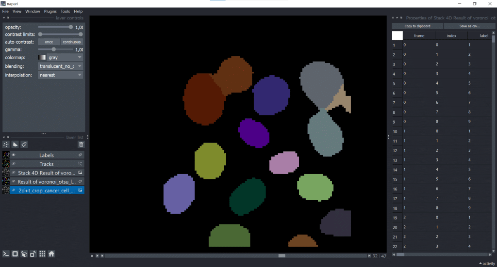
Exploring image dimensions with napari-layer-details-display

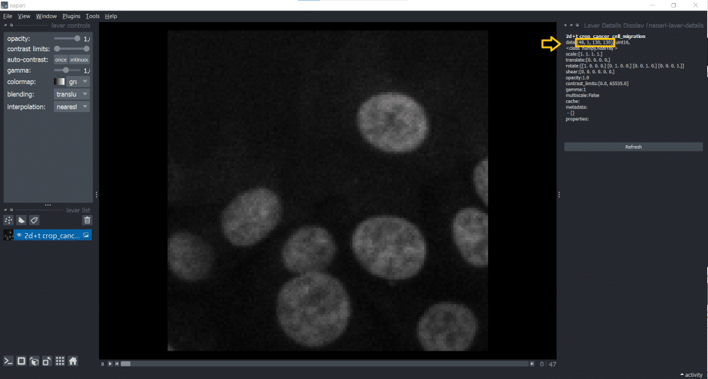
Before we can start tracking, we need to find out which shape our image has. Therefore, we go under Plugins → Layer Details Display (napari-layer-details-display). This will display image properties (e.g. shape and scaling):

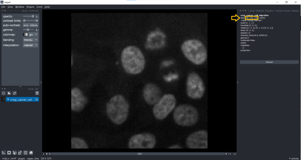
Layer Details Display widget displays properties of the selected object in the label list (blue = selected)

Now, we know that our image is a 3D stack with [48, 130, 130] corresponding to [t,y,x]. This might lead to a confusion between t and z dimension later, but we can change this easily using the napari-time-slicer.

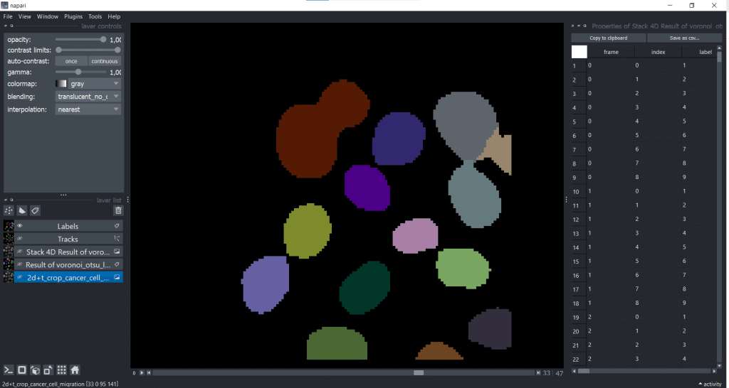
Changing image dimensionality with the napari-time-slicer

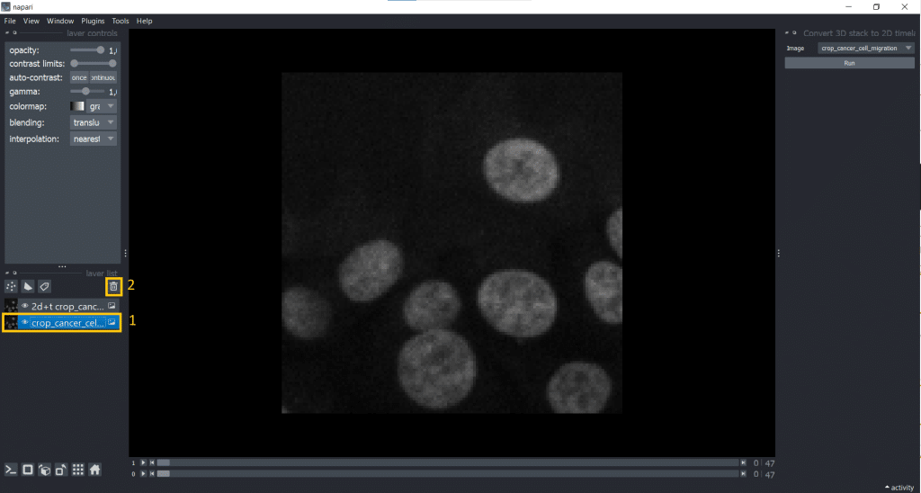
The napari-time-slicer allows processing timelapse data timepoint-by-timepoint. In this case, we will use it to convert our input image from [t,y,x] into [t,z,y,x] to avoid any confusions between t and z dimension. Lets have a look under Tools → Utilities → Convert 3D stack to 2D timelapse (time-slicer). When hitting the Run-button, the plugin creates a new layer called 2D+t <original name>.

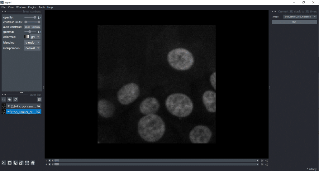
Convert 3D stack to 2D timelapse widget helps converting `[t,y,x]` into `[t,1,y,x]`.

Afterwards, it makes sense to delete the original image from the layer list to avoid confusion. Just select it in the layer list on the left and hit the trashbin icon.

Deleting the original image layer from the layer list to keep an overview.

If we now check our image shape again using napari-layer-details-display, we see our conversion from [t,y,x] into [t,1,y,x] was successful. Here, 1 stands for our one z-slice.

A general remark: You can save output at any time to disk by selecting the layer of interest and under File → Save Selected Layer(s) selecting a place to store the image. Now, we are ready to track!

Coordinate-based tracking with napari-laptrack

We will explore how to perform coordinate-based tracking with spot-detection and linking.

Segmentation with Voronoi-Otsu-Labeling (clesperanto)

For this purpose, we need a segmentation result. When it comes to segmentation algorithms, we have a variety of choices (see Napari-hub). Here, we will use Voronoi-Otsu-labeling as implemented in clesperanto under Tools → Segmentation/labeling → Voronoi-Otsu-labeling(clesperanto). We choose spot sigma = 5 und outline sigma = 3.

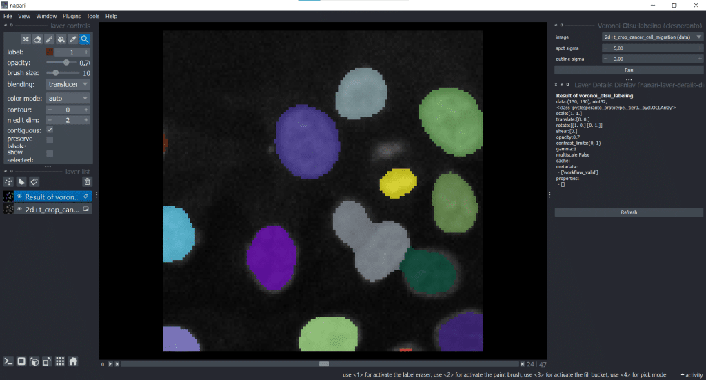
Voronoi-Otsu-Labeling widget of the napari-pyclesperanto-assistant and Label Details Display widget

Be aware that now only the currently displayed timepoint is segmented and not all timepoints. You can also double-check in napari-layer-details-display and will see that our segmentation result has an image shape of [y,x].

Tracking with napari-laptrack

Now, we are ready to track using napari-laptrack. The coordinate implemented in napari-laptrack is the centroid. We can find this centroid-based tracking option under Tools → Tracking → Track labeled objects (centroid-based, LapTrack). Therefore, we need to select an image_layer and a labels_layer. Next, hit the Run button as there are no parameters we can/ need to tune.

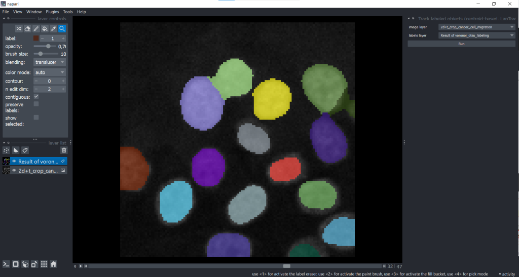
Track labeled objects widget of napari-laptrack

After the tracking process is finished, multiple layers were generated by the plugin:

Output generated by napari-laptrack: stack 4D result of Voronoi-Otsu-Labeling, tracks layer, labels and table with properties

In the following paragraphs, the different layers will be explained in more detail.

1. Stack 4D Result of Voronoi-Otsu-Labeling

Basically, the segmentation result that we produced before is only one timepoint at a time, so shaped [y,x]. The plugin now converts this 2D image into a 4D stack by segmentating the whole time-lapse dataset. The result is a 4D stack shaped [t,1,y,x].

As you may have recognized, for the image layer we had to do this step ourselves. But for the labels layer it is already implemented in the plugin.

2. The Tracks layer

The napari Tracks layer visualizes the positional change of objects, in this case of the labels centroids, over time. Hereby, only a certain range of timepoints close to the current timepoint is visualized and not the whole track. This so called “fading tail” visualization allows us to keep an overview when looking at the Tracks layer. If we select in layer list the Tracks layer, we can fine-tune visibility and coloring of the tracks. They are listed under layer controls. In my opinion, very handy is:

color by different properties: mapping colors to different tracking properties
changing the tail width
changing the tail length
show ID of the individual tracks (= number of the track)

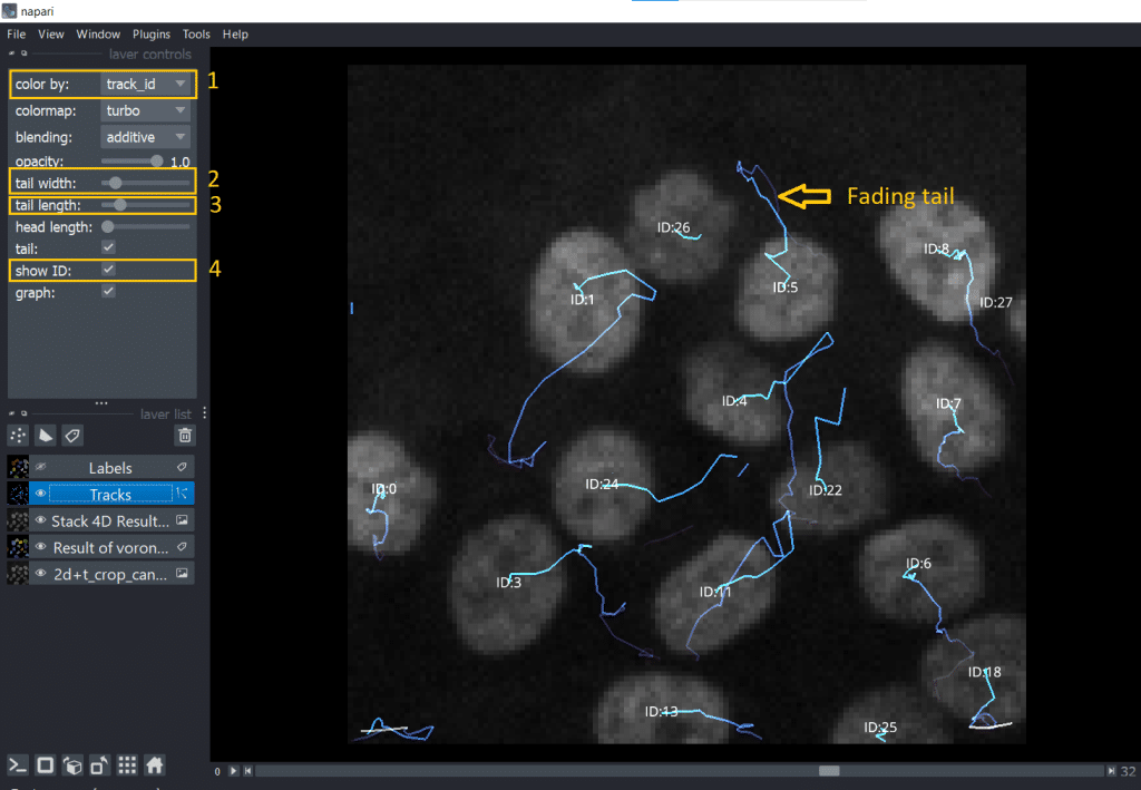
The Tracks layer in napari and how to fine-tune it

Alternatively, we can also hover over the tracks with the mouse. The Track ID is then displayed in the bottom left corner of the napari window.

3. Labels – The Track ID image

In the layer called Labels the objects have the same label number/ color. For better understanding, see these two consecutive frames:

In the track ID image, the objects keep the same label number/ color over time.

4. Table with properties

Furthermore, we get a table with different properties which were measured on our 4D Stack of our Voronoi-Otsu-Labeling result.

btrack

Now, we want to try btrack, another tracking tool which was developed to monitor multiple generations.

Personal preference: Run btrack from a jupyter notebook. From my point of view, it is easier to handle and tune from a notebook. You can find a demo notebook here.

If you don’t want to work in a jupyter notebook, you can also run it directly in napari. For this, we need a [t,1,y,x] input as label image. We can get such a 4D stack for our Voronoi-Otsu-labeling result by selecting Tools → Utilities → Convert to file-backed timelapse data and choosing our label image:

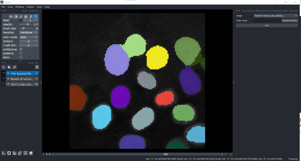
Convert to file-backed timelapse data widget helps converting `[y,x]` into `[t,1,y,x]`

Basically, we now did a conversion step manually that napari-laptrack was able to do automatically. Afterwards, it makes sense to delete our original Voronoi-Otsu-Labeling result to avoid any confusions. Now, both image and label image are [t,1,y,x].

We can now find btrack under Plugins → Track (btrack):

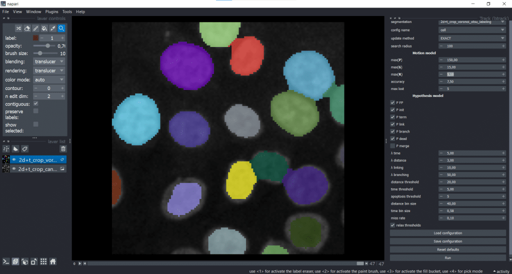
On the right, we can see the graphical user interface of btrack containing different parameters that we can tune. For now, we will leave everything at the default settings and hit the Run button. The btrack developers plan to write a how-to-guide for the parameter tuning. If you have any suggestions/ wishes for this guide, questions are collected here.

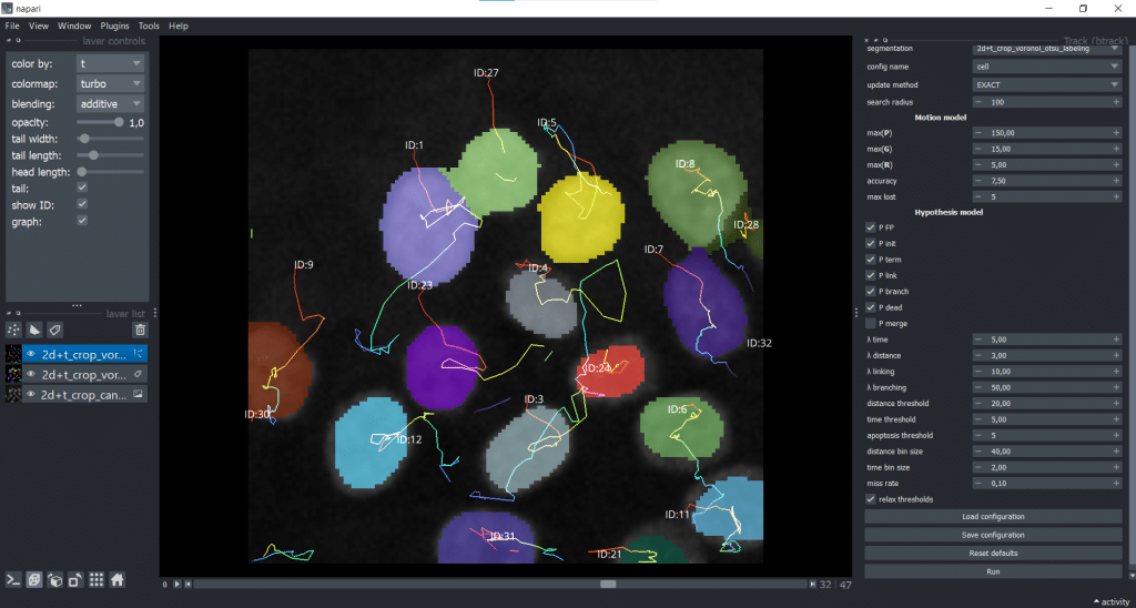
We receive a napari Tracks layer as output. As you can see, I ticked the show ID checkbox and chose to color by time (t).

napari-laptrack and btrack in comparison

We have now tried two different napari-plugins and have seen their output. In the following table, see some personally noticed differences:

category	napari-laptrack	btrack
input	image	label image, image only needed when measuring intensity
input dimensionality	image: `[t,z,y,x]` label image: `[y,x]`	can handle different image dimensionalities (e.g. `[t,y,x]` or `[t,z,y,x]`) when parameter `volume` is adjusted (see jupyter notebook)
run from … (personal recommendation)	napari	jupyter notebook
segmentation features	not implemented, but can be connected to napari-skimage-regionprops	segmentation can be connected to skimage regionprops using `utils.segmentation_to_objects` (see jupyter notebook)
tracking features	/	/

Comparison of napari-laptrack and btrack

Quality assurance of tracking results

But how can we find out if our tracking result makes sense?

In general, keep in mind that there is an error propagation over time: the more timepoints we analyse, the worse the tracking result is going to be (see explanation).

One idea would be to do a plausibility check. We could check if the number of cell divisions makes sense in a given time. Besides the number of splits, we could also investigate tracking features like position, velocity or displacement rate. For this, determining the meaningfulness of the tracking result requires knowledge on our dataset.

Another approach would be to compute lineage trees out of the tracking results and look for unlikely events like track merging or gaps within individual tracks.

A third option would be to track forwards and backwards in time. This would lead to one tracking result with split events (tracking forward) and one tracking result with merge events (tracking backward) and check if the result is similar. If something is wrong, then at least one of the results must be wrong.

Another idea would be correlation analysis of the tracking tables of manual and automated tracking. This only works if they have similar row sequence, so I am unsure if this is feasable.

Also, we could manually track our dataset (or a crop) and compare the manual tracking result to our automated tracking result. This approach can be very time-consuming depending on the size of the dataset. But we could visually compare lineage trees of the manual and automated tracking.

Manual vs. automated tracking

We have seen already how we can automatically track, but there is also the option of manual tracking.

Def. Manual tracking: Manual tracking describes annotating a video frame-by frame by hand to derive the positional information of the objects over time.

Manual and automated tracking have both advantages and disadvantages to them.

category	manual	automated
advantages	potentially more correct, flexible and adaptable	reduced time and effort, consistent and reproducible results, potential for high-throughput analysis
disadvantages	labour-intensive, time-consuming, subjective bias	sensitivity to noise and image quality, difficulty with complex cell dynamics, may require manual validation/ correction

Advantages and disadvantages of manual and automated tracking

Unfortunately, it is hard to manually track in napari at the moment. But it would be interesting to investigate whether it’s faster to manual postprocess after automated tracking or track manually in the first place.

Feature requests

This brings us to feature requests for tracking plugins. Many of the shown tools are in experimental developmental phase. You can find out about the status of different plugins on napari-hub. Typical stages are pre-alpha, alpha, beta, release candidate and stable release. Please treat the generated results with care. If you are interested in the different phases of software development, you can read more about developmental statii of software.

Useful features that could still be implemented are from my point of view:

Idea	Corresponding GitHub Issue
Enable manual tracking	Lin k
Measuring tracking features (e.g. velocity)	Link
Visualizing selected tracks and the corresponding feature table row	Link
Enable manual postprocessing of the tracks (adding and removing tracks)	Link, see laptrack example notebook
Enable tracking 3D+t dataset in napari-laptrack	Link
How-to-guide for btrack model parameter tuning	Link

Feature requests: in case of interest to you leave thumbs up under the related GitHub Issues, add ideas there or send a pull request if you want to solve them.

Conclusion

We saw that cell tracking has many facets to it and is a very interesting research field which can also get complicated. Therefore, it makes sense to first think about your target measure and whether tracking is necessary for your project, before starting to go down the tracking road. For example if we want to determine the cell count, it would be easier to determine the nuclei than segmenting and tracking (see also mountain metaphor). Also distribution analysis could be of interest, e.g. if shape distributions over time are investigated.

As functionality of most of the shown tracking napari-plugins is limited, their results should be treated carefully.

Feedback welcome

Some of the napari-plugins used above aim to make intuitive tools available that implement methods, which are commonly used by bioinformaticians and Python developers. Moreover, the idea is to make those accessible to people who are no hardcore-coders, but want to dive deeper into Bio-image Analysis. Therefore, feedback from the community is important for the development and improvement of these tools. Hence, if there are questions or feature requests using the above explained tools, please comment below or open a thread on image.sc. Thank you!

Acknowledgements

I want to thank Dr. Robert Haase, Dr. Yohsuke T. Fukai, Dr. Kristina Ulicna and Prof. Alan R. Lowe as the developers behind the tools shown in this blogpost. This project has been made possible by grant number 2022-252520 from the Chan Zuckerberg Initiative DAF, an advised fund of the Silicon Valley Community Foundation. This project was supported by the Deutsche Forschungsgemeinschaft under Germany’s Excellence Strategy – EXC2068 – Cluster of Excellence “Physics of Life” of TU Dresden.

Reusing this material

This blog post is open-access, figures and text can be rused under the terms of the CC BY 4.0 license unless mentioned otherwise.

(2 votes, average: 1.00 out of 1)

Tags: microscopy, image analysis, image data science, napari, Tracking, cell tracking
Categories: Bio-image Analysis with Napari, Default, How to

Get involved

Create an account or log in to post your story on FocalPlane.